Overview
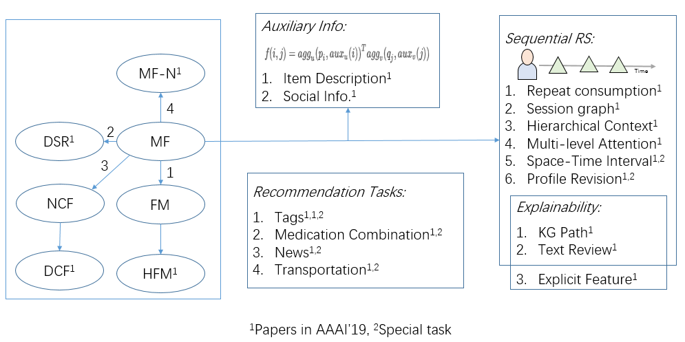
Introduction
Explainability
Recently, the recommendation community has reached a consensus that accuracy can only be used to partially evaluate a system. Explainability of the model, which is the ability to provide explanations for why an item is recommended, is considered equally important.
Papers like follows:
- Explainable Reasoning over Knowledge Graphs for Recommendation: Use knowledge graph(KG) info for explainability. Select the most related path in KG as the explanation.
- Explainable Recommendation Through Attentive Multi-View Learning: Construct a hierarchical (explicit) feature (e.g. meat, seafood and so on) tree for explainability. Select the most related features as explanation.
- Dynamic Explainable Recommendation based on Neural Attentive Models: Generate dynamic explanations at different time for a user by using GRU. An explanation is the most related sentence in the review of the recommended item.
Sequential Recommendation
Different from traditional MF that treats users and items equally, the methods model the interactions between users and items as a number of historical interaction sequences of users. Then focusing on the sequential interactions of users, some methods was proposed to analysis the phenomenon like long-term interests, drifted interests, repeat consumption and some other task-specific aspects. The tasks include next item (basket) prediction (like POI), session recommendation.
- A Repeat Aware Neural Recommendation Machine for Session-based Recommendation: Emphasize the importance of repeat consumption.
- Session-based Recommendation with Graph Neural Networks: Model item transitions in sessions as a Graph.
- Hierarchical Context enabled Recurrent Neural Network for Recommendation: Emphasize global long-term interests, local sub-sequence interests and the temporary interests of each transition in a sequence.
- A Spatio-Temporal Gated Network for Next POI Recommendation: Emphasize the influence of spatio-temporal intervals between check-ins for POI recommendation.
- Multi-order Attentive Ranking Model for Sequential Recommendation: Emphasize the difference of individual-level and union level item relevance.
Cross Domain Recommendation
- Deeply Fusing Reviews and Contents for Cold Start Users in Cross-Domain Recommendation Systems: User more kinds of auxiliary info.
- From Zero-Shot Learning to Cold-Start Recommendation: Use ZSL method to solve CSR problem
Improve Basic Methods
- Holographic Factorization Machines for Recommendation: Improve Factorization Machine (FM) with convolution operation.
- Non-Compensatory Psychological Models for Recommender Systems: A novel method following the non-compensatory rules in consumer psychology while all traditional latent factor models fall into category of compensatory rules.
- Discrete Social Recommendation: To speedup models with quantization while maintain the performance as possible as we can.
- A Unified Framework of Representation Learning and Matching Function Learning in Recommender System: A combination of two kinds conventional methods: representation learning based methods like MF and matching function learning based methods like NCF.
Specific Tasks
These methods utilize the information in some specific scenarios.
- POI recommendation as above
- DAN: Deep Attention Neural Network for News Recommendation: Do a specific task with a complex combination of popular networks (actually news is just treated as text). The emphasized point is still the order info that has been studied for general recommendation over and over again.
- Graph Augmented MEmory Networks for Recommending Medication Combination: Also a specific task that recommends medication combination. The point is to process patient health history and drug-drug interactions with proper techniques.
- An Integral Tag Recommendation Model for Textual Content: The authors emphasize three aspects of tag recommendation that impact the accuracy: 1) sequential text modeling. 2) tag correlation. 3) content-tag overlapping.
- Hashtag Recommendation for Photo Sharing Services: Utilize info of image, text and personalized habits.
- Joint Representation Learning for Multi-Modal Transportation Recommendation: Multi-Modal Transportation Recommendation. The main contribution is to format this problem while the method is simple.
- Hierarchical Reinforcement Learning for Course Recommendation in MOOCs: Use RL to revise user profiles by removing the noisy courses instead of assigning an attention weight to each of them. The basic idea is independent from MOOCs but the author use info only in MOOCs to present state in RL.
Others
- A Collaborative Ranking Method for Content Based Recommendation: Follow a traditional line that generates item embedding from auxiliary info and then combine it with MF like $u_i^T(v_j + embedding(doc_j))$
- Modeling Influential Contexts with Heterogeneous Relations for Sparse and Cold-Start Recommendation: A general formation of recommendation with user-item interaction, user-user relation(social relation), item-item relation.
- Evaluating Recommender System Stability with Influence-Guided Fuzzing: Predefine some modifications to modify the dataset and then evaluate the stability of some classical recommendation method.
- Large-scale Interactive Recommendation with Tree-structured Policy Gradient: Construct all items as tree to reduce the time complexity of choosing an item from all items.
- Meta Learning for Image Captioning
- From Recommendation Systems to Facility Location Games: An interest aspect for recommendation problem. The authors design a Mediator (for service providers) to direct what the content providers(e.g. blog/video publishers) should provide to achieve overall higher social welfare while intervene as little as possible. The introduction of method is omitted for it is more related to social science and a bit complex.
- Multi-Level Deep Cascade Trees for Conversion Rate Prediction in Recommendation: A problem related to recommendation. The problem want to predict conversion rate when users have clicked and viewed recommended items. Briefly, take Taobao for an example, conversion means users bought the recommended item after they clicked and viewed the item.
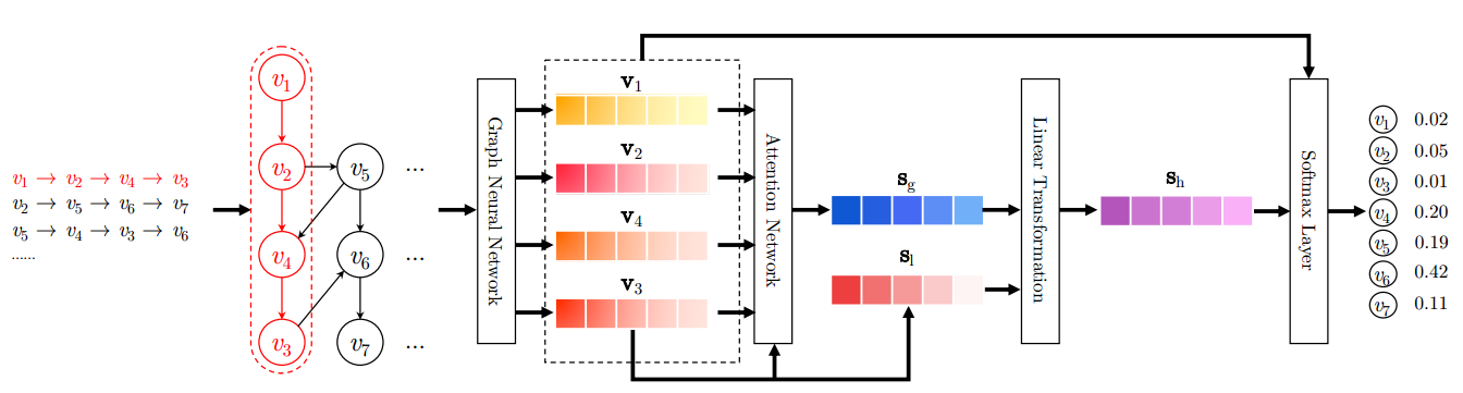
Session-based Recommendation with Graph Neural Networks
Problem: Session Recommendation
Gap: Transitions among distant items are often overlooked by previous methods.
Method: Use Graph to model item relation in sessions and utilize Graph Neural Networks to capturing transitions of items and generate accurate item embedding vectors. For example, as follows, the three sessions are constructed as a graph.
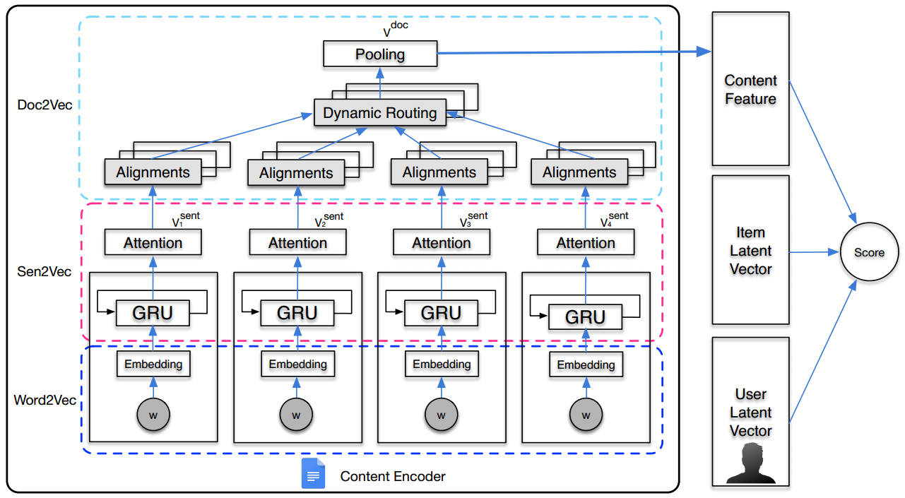
A Collaborative Ranking Method for Content Based Recommendation
Problem: A traditional line that uses auxiliary information to enrich item embedding based on MF. The general score function for user $i$, item $j$ and auxiliary info $doc_j$ is as followings:
$$
f(i,j,doc_j) = p_i^T(q_j + g(doc_j))
$$
where $g(.)$ is the encoding function.
Gap: For function $g(.)$, some methods ignore the order of words, while others fail to identify the high leveled topic info.
Method: An encoding function based on GRU(capture order) and multi-head attention mechanism(model topic info).
A Nice Attention Introduction: https://lilianweng.github.io/lil-log/2018/06/24/attention-attention.html
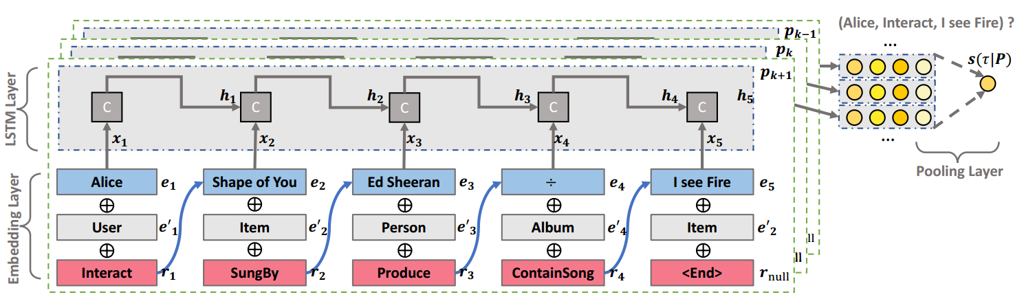
Explainable Reasoning over Knowledge Graphs for Recommendation
Problem: recommendation with explainability, using KG specifically.
Gap: The connectivity information in KG can help to endow recommender systems the ability of reasoning and explainability. However, some traditional methods(use meta-paths) need domain knowledge to predefine meta-paths, while others(embedding based, like using TransE) are less explainable.
Method:
Model user-item interaction $(u, i)$ as KG triplet relation $(u, interact, i)$.
For each $(u,i)$, select all paths from user node $u$ to item node $i$, denoted as $P(u,i) = {p_1, p_2, …, p_K}$
The score function from user $u$ to item $i$ is modeled as:
$$
\hat{y}{ui} = f{\Theta}(u,i|P(u,i))
$$Use LSTM to model the preference of each path and use a weighted pooling layer(not attention) to calculate the final preference and estimate the importance of each path.
Weighted Pooling Layer:
For each preference $s_k$ outputted from the LSTM layer, the weighted pooling layer is defined as follows:
$$
g(s_1, s_2, …, s_K) = log[\sum_{k=1}^K \exp (\frac{s_K}{\gamma})]
$$
where $\gamma$ is a hyper-parameter to control each exponential weight and the path importance is estimated from the gradient on each path preference:
$$
\frac{\partial g}{\partial s_k} = \frac{\exp (s_k/ \gamma)}{\gamma \sum_{k^{‘}} \exp (s_{k^{‘}}/\gamma)}
$$
Finally, the score function is
$$
y_{ui} = \sigma(g(s_1,s_2,…,s_K))
$$
From Zero-Shot Learning to Cold-Start Recommendation
Problem: Cold-start Recommendation(CSR)
Gap: no gap but a novel view in light of Zero-Shot Learning(ZCL). Actually, I am not used to this kind of writing pattern.
Challenge to formulate CSR as a ZSL problem:
- Domain shift problem: the data distribution is not same as in ZSL
- Data sparsity: the interactions in recommendation domain is very sparse.
- Efficiency.
Method: Use a Linear Low-rank Autoencoder to learn a transform matrix $W$ that transfer user behavior matrix $X$ into user attributes matrix $S$ as follows:
$$
\min_{W}|| X - W^TWX||F^2 + \beta rank(W), s.t. WX = S
$$
Then, for new users, we can estimate their potential user behavior matrix $X{new}$ as
$$
X_{new} = W^TS_{new}
$$
My concern is how the autoencoder or low-rank constraint solve the data sparsity problem in Recommendation domain. In ZSL, each $X$ is an image with enough info. However, in RS, each $X$ is an interaction matrix which is very sparse and in total, there is only one large matrix with the user number as row number and item number as column number as train data. Compare to ZSL, the train dataset is also very small.
A similar low-rank Autoencoder for ZSL in IJCAI’18: Zero Shot Learning via Low-rank Embedded Semantic AutoEncoder
Meta Learning for Image Captioning
Problem: Image caption
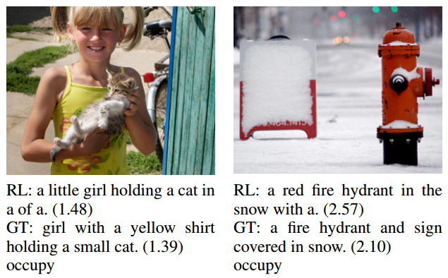
Gap: reward hacking problem in RL. Shown in the following figure, the reward (digit next to the caption) of caption generated by RL is even higher than the ground truth (GT) caption while the caption quality is actually not.
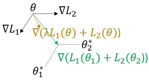
Method: Utilize the power of meta-learning to ensure the correctness and distinctiveness of the generated captions(by RL reward) and optimize the evaluation metrics(by maximizing the likelihood of the ground truth caption). Shown in the following graph, the meta-learning objective(marked in green) could the learn $\theta$ that is optimal to adapt both tasks while just adding RL reward $L_1(\theta)$ with maximize likelihood target $L_2(\theta)$takes a gradient in between (marked in brown).
The idea behind this work may suggest that we should use meta-learning optimization method to substitute trivial aggregation of different losses in all kinds of works if there is the similar hacking problem in the corresponding domains.
Explainable Recommendation Through Attentive Multi-View Learning
Problem: recommendation with explainability
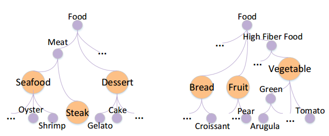
Gap: On one hand, some deep learning-based methods lack of explainability. On other hand, other shallow models lack of an effective mechanism to model high-level explicit features which limits their accuracy. What’s more they can’t identify hierarchical interests. As shown in the following graph, previous works can not identify whether a user is interested in lower-level features such as $\textit{shrimp}$ or higher-level features like $\textit{seafood}$.
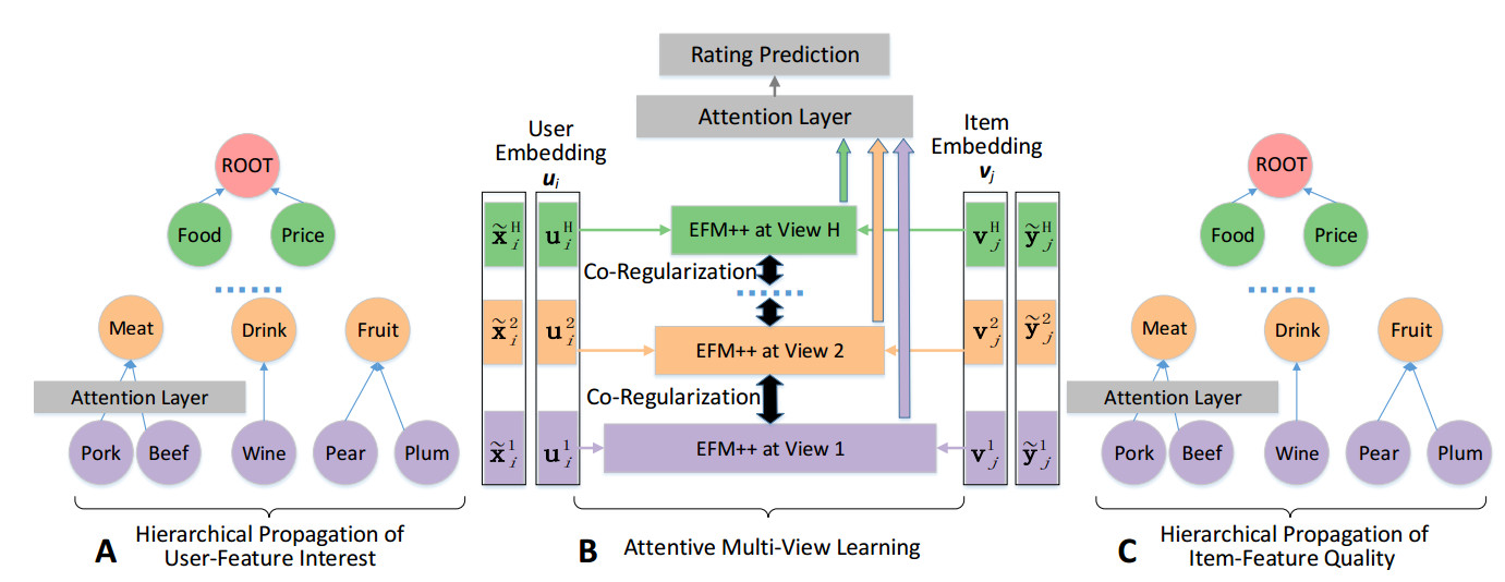
Method: feed the model with the hierarchical features information. An overview is as follows.
- Build an explicit feature hierarchy $\gamma$ with in total $L$ features and $H$ layers from the collected data like Microsoft Concept Graph. Pretrain with the graph to get the embedding $e_i$ of each feature node.
- For a user $i$, collect his explicit user-feature interest $x_i$ from his reviews. $x_{il}$ indicates the frequence of the feature $F_l$ being mentioned by the user.
- propagate the feature-interest on the tree to get more proper interest $\hat{x_i}$ to let each interest on the feature node contain the interests on its sub-nodes.
- For items, build their features denoted as $\hat{y_j}$ from product introduction in a similar way.
- Attentive multi-view learning with the ratings and collected features as supervising info. Each user and item has an implicit feature and an explicit feature. Both features need fit ratings based on MF while the explicit features need also fit collected features with a linear transform and L2 loss.
The overall process is as follows.
Then for explainability, the method utilize the feature hierarchy $\gamma$ and the trained model to select some important features as reason of recommendation.
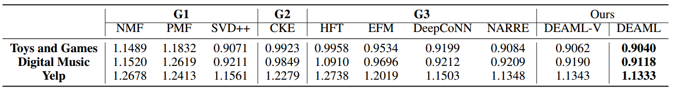
Additionally, from the experimental results shown in the following figure, we can see SVD++ performs well with RMSE metric and even performs better than some deep models likes DeepCoNN and NARRE that using review info. The phenomenon should be discussed more detailly.
Dynamic Explainable Recommendation based on Neural Attentive Models
Problem: recommendation with explainability
Gap: Most previous works represent a user as a static latent vector($most$ is a good word). More importantly, the explanations provided by these models are usually invariant.
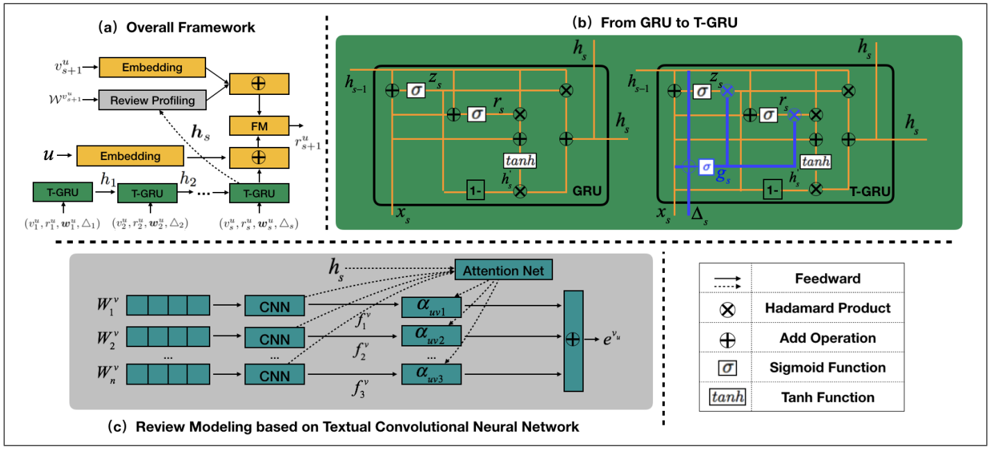
Method: Use GRU to model dynamic interest of users. Add a time gate to GRU to use the message of time interval. For example, a user tend to have similar preferences within a short time, while large time gap may have more opportunities to change user interest. For an item, use the hidden state $h_s$ of GRU at current time as the user’s interest to select the most related sentence in the reviews as explanation by making use of attention mechanism. The general process is shown in following figure.
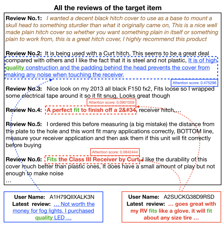
An example of explanation is shown as follows.
DAN: Deep Attention Neural Network for News Recommendation
Problem: News recommendation (next item recommendation)
Gap: They usually fail with the dynamic diversity of news and user’s interests, or ignore the importance of sequential information of user’s clicking selection. (This is obviously a false assertion for general recommendation)
Method: Combination of CNN, RNN and Attention Mechanism.
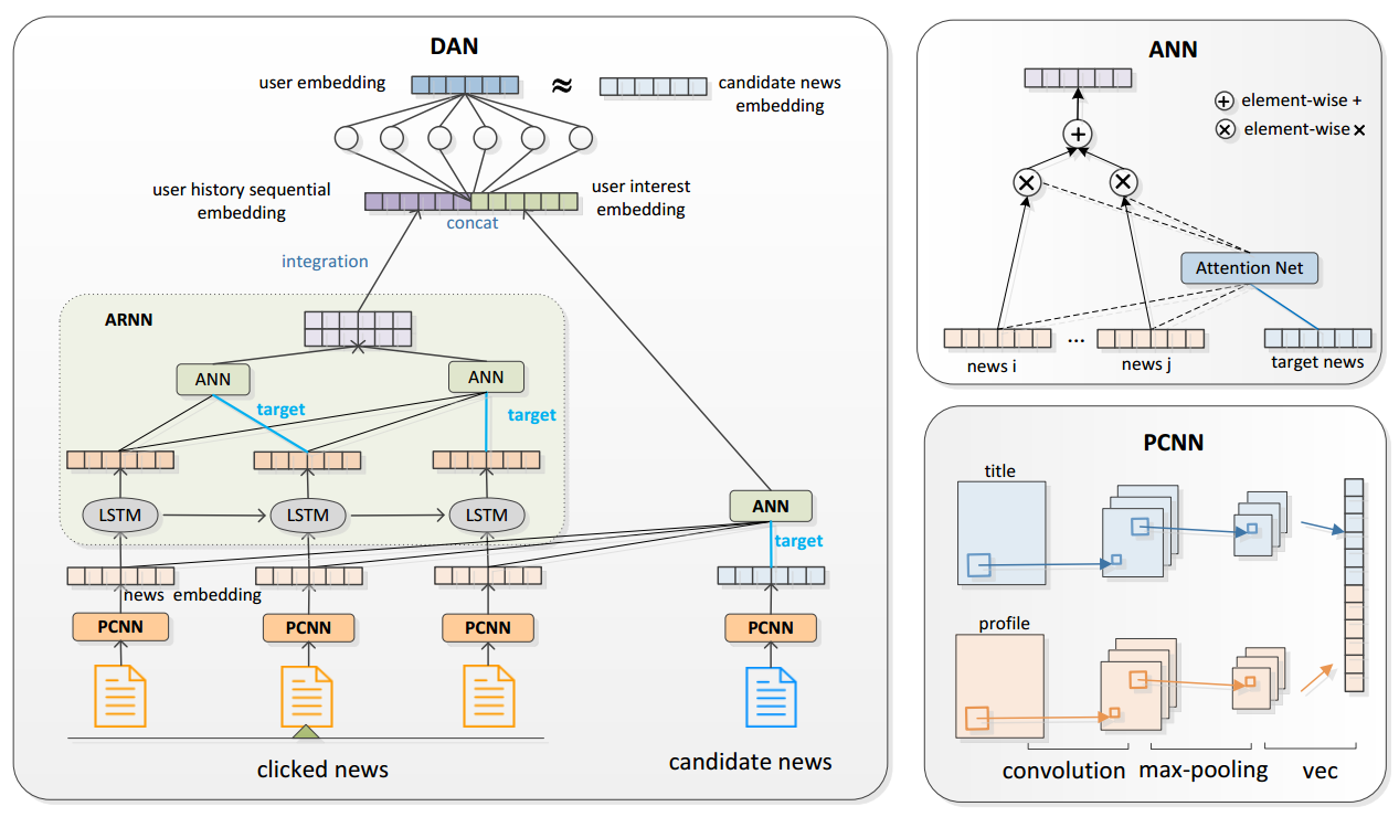
As shown in the above figure, the process is summary as:
Use two CNN(PCNN) to extract embedding of news with title and profile parts.
Use LSTM and Attention to learn a user’s embedding with a sequence of clicked news.
Score function is based on similarity between user embedding and candidate news embedding as follows. The $cosine$ function is calculated by the inner product of two vectors which is the same with MF but with different name.
$$
P = cosine(\hat{I}_t . I_t)
$$
A Repeat Aware Neural Recommendation Machine for Session-based Recommendation
Problem: session recommendation
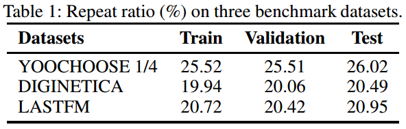
Gap: propose a novel repeat consumption phenomenon where the same item is re-consumed repeatedly over time. The following table shows the repeat ratio in three public datasets. However, no previous works have emphasized repeat consumption with neural networks. (Multi-armed bandit problem has been studied for a long time to solve the repeat-explore dilemma for general recommendations.)
Method:
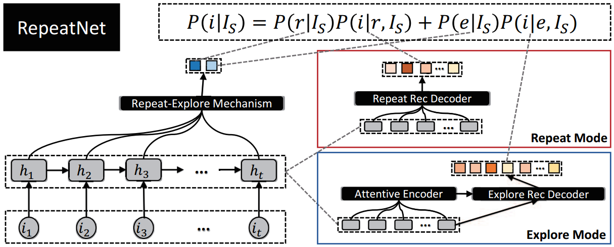
As shown in the above figure, the process is summarized as:
- Use GRU to encode the session sequence of a user.
- Use attention mechanism to merge all hidden states with the last hidden state as attention point. Then use a dense network to transform the merged vector into a two dimension vector with the first value as the probability of repeat and the other as the probability of explore
- For repeat mode, decode the hidden states to calculate score for each item (new items get 0 point)
- For explore mode, decode the hidden states with attention to calculate for each item (old items get 0 point)
- Use the score and whether the item is new as supervising info to train model with a negative log-likelihood loss and a logistic loss.
Hierarchical Context enabled Recurrent Neural Network for Recommendation
Problem: Next-item recommendation
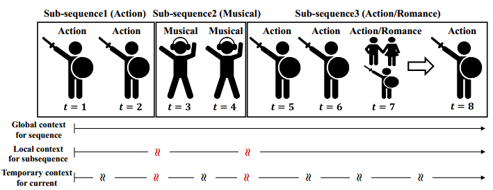
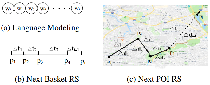
Gap: Emphasize long-term interests, local sub-sequence interests and temporary interests of each transition which are shown in the following graph while all these interests have only been partially reflected in most previous works.
Method: (the authors assume each sequence should be longer than 10 in experiments)
Traditional LSTM process is shown as follows:
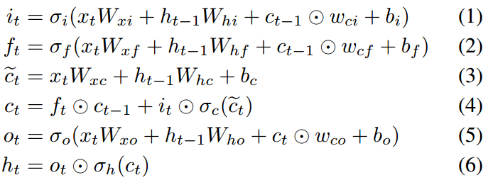
The authors propose to use cell state $c_t$ to present the local-sub sequence interests and use hidden state $h_t$ to present temporary transition interests. However, in traditional LSTM, $h_t$ are only directly dependent on $c_t$, there is little difference between them. Besides the long-term interests are neglected if $c_t$ is treated only as local interest. So, the author modify to LSTM to let $h_t$ more independent and add a memory network to keep long-term interests. The process is shown as
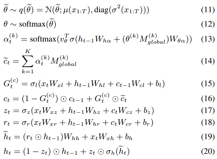
where the parameter $\theta$ are trainable parameter $\theta$ for attention mechanism. Then in each transition, the influence of global long-term interests is considered.
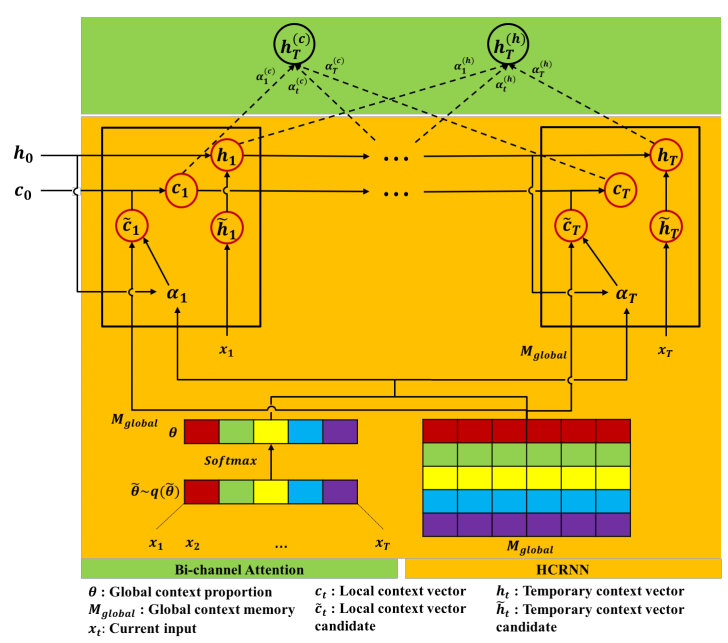
The general process is shown in the following graph in which other tricks like bi-channel attention for prediction to focus on all interests are simply demonstrated.
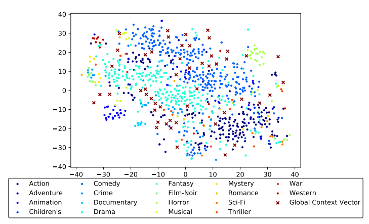
One way to demonstrate global interests is shown in the following graph from which we can see global context vector cover the most of the items.
A Spatio-Temporal Gated Network for Next POI Recommendation
Problem: POI recommendation (next item prediction)
Gap: Most previous recommendation methods don’t consider both time intervals and geographical distances between neighbor items that are shown in bellowing figure. And some other methods may fail to model spatial and temporal relations of neighbor check-ins properly (see paper for more detail discussion).
Method:
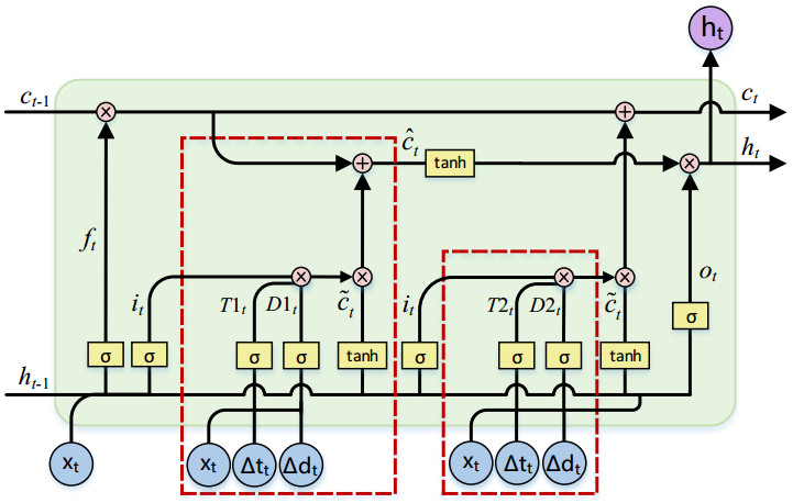
Shown in the above figure, based on LSTM, the authors also add two time interval gates and two distance gates (no direction info) besides the input gate.
Gates $T1, D1$ are used to filter new information considering influence of time interval and distance and then the filtered information is transferred to the hidden state and finally influences the next recommendation. Gates $T2, D2$ are used in a similar way for estimating new cell state.
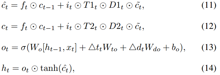
Multi-order Attentive Ranking Model for Sequential Recommendation
Problem: Next item recommendation
Gap: Except for the individual-level relevance, union-level item relevance also influence a user’s interactions. For example, buying eggs, milk, and butter together indicates a higher probability of buying flour than eggs, milk or butter individually. However, most previous works neglected the union-level relevance and others didn’t model it well (see paper for more detail discussion). The following figure shows two kinds of relevance.
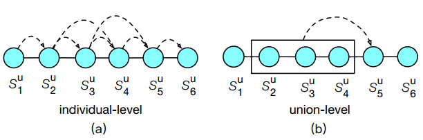
Method: To predict the score of item $j$ for a user $u$, the authors also directly add the influence of the items, denote as a set $S_{t-1,n}^u$, that the user has interacted with recently. Then the final prediction is estimated as
$$
\hat{y}_{u,j} = p_uq_j^T + F(u, S_{t-1,n}^u)m_j^T
$$
Then the point is how to model the union-level preference $F(u, S_{t-1,n}^u)$.
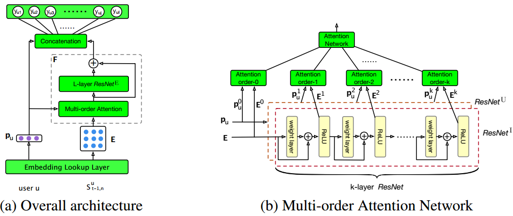
Generally, shown in the left of the above figure, the authors use the user feature $p_u$ as the attention point to decide the weight of each item $S_{t-1,n}^u$ with as special Multi-order Attention Network (see paper for detail). The the output, denoted as $e_c$, of the Attention Network could regard as the individual-level influence of the items in $S_{t-1,n}^u$ to the target item $j$ with each item with different attention weight. To capture the union-level influence, the authors add a L-layer ResNet to fuse the influence in $e_c$ to a high-level feature, denoted as $h_L$. Finally the feature $F(u, S_{t-1,n}^u)$ is $e_c + h_L$.
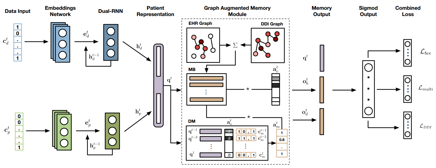
Graph Augmented MEmory Networks for Recommending Medication Combination
Problem: Recommend medication combination, a special specific task
Gap: Existing approaches either do not customize based on patient health history, or ignore existing knowledge on drug-drug interactions (DDI) that might lead to adverse outcomes.
Method: The method is a bit complex in actual. Briefly:
Use Graph to represent the DDI relation and the estimated drug combination relation from patient health history.
Use GCN (Graph Convolutional Network) to learn Graph node representations and then format them as two memory networks: 1) memory bank (MB): the key and value are both node embeddings. 2) dynamic memory (DM): the key is embedding of a user’s historical diseases (learned as follows) before current time and the value the the corresponding medication combination.
Use RNN to learn embeddings of a user’s historical diseases at each time, denoted as $q_t$.
Use $q_t$ as query vector to query the two memories built as above and use the collected memory to do a multi-label classification to recommend medication combination
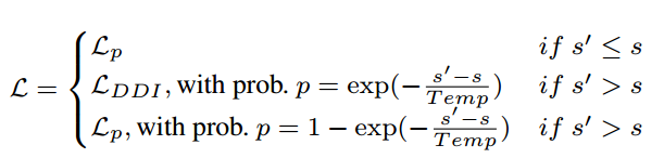
Besides the traditional multi-label classification loss, the authors also add a DDI loss to avoid drug-drug -interactions like follows where $A_d[i,j] = 1$ if drug $i$ has an interaction on drug $j$
$$
L_{DDI} = \sum_t^T \sum_{i,j}(A_d \odot (\hat{y}_t^T\hat{y_t}))[i,j]
$$Additionally, the authors use a special combined loss functions in medication instead of weighted aggregation
Finally, the overall architecture is shown in the following figure. A users’ historical disease consists of two parts. One is the diagnoses code $c_d^t$ and the other is the procedure code $c_p^t$
Deeply Fusing Reviews and Contents for Cold Start Users in Cross-Domain Recommendation Systems
Problem: Cross-Domain Recommendation for cold-start users.
Gap: Most existing cross-domain recommendation works still do not take full consideration of different kinds of valuable side information (In this paper, there are two kinds of information: review texts and item contents).
Method:
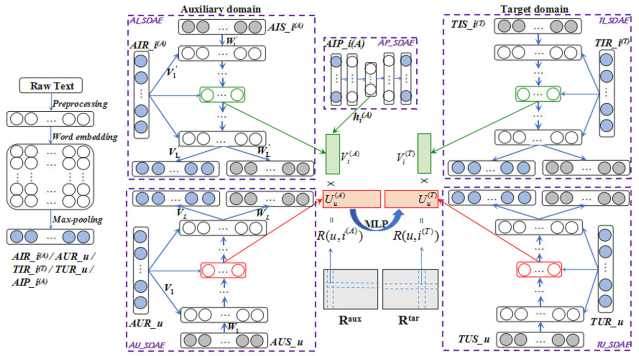
The framework is shown as above, the brief process is summarized as:
- For both domain, the text info of a user is all of his review texts, the text info for a item is all reviews on it. Besides, in auxiliary domain, the text info of item also includes item contents.
- Use Stacked Denoising Autoencoders to encoding a user according to his/her ratings on all items with the text info as a side info (like AUR_u in the left bottom). Learn the representations of items in a similar way except for items in auxiliary domain that also utilize item contents (AIP_i(A) in upper center)
- Use MF to predict ratings in both domain
- Use MLP to transfer the features in auxiliary domain to target domain.
My concern is that the MLP part only tunes parameters of MLP based on this transform method. In another word, the features of users and items should be pretrained. Then the pretraining of $U$ and $V$ to let them prepared for the transform part will be a hard work utilizing only the sparse rating matrices. Instead, the pretraining works in other domain like NLP and CV usually need a very large dataset.
Discrete Social Recommendation
Problem: social recommendation
Gap: With traditional methods like MF, the large volume of user/item latent features results in expensive storage and computation cost, particularly on terminal user devices where the computation resource to operate model is very limited. Besides, some quantization methods(use lower precision values, e.g. 2-bit int vector instead of 32-bit float vector) would lose accuracy after the model has been trained.
Method: To learn binary vector as features of users and items.
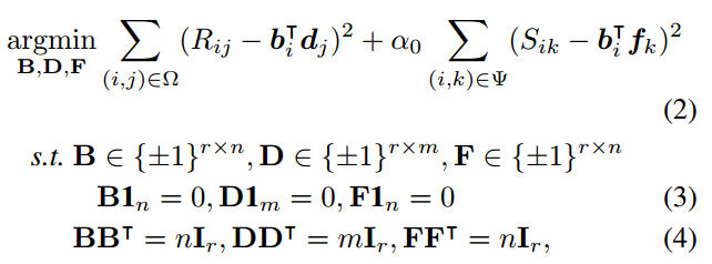
Shown in the above figure, the idea is simple. All feature vectors $b_i, d_j, f_k$ are binary vectors. Here $S$ is the social relation between users and $f_k$ is a third latent feature (different from $b_k$).
The challenge is how to optimize this problem. The problem is a little similar with NMF, but this problem has much more constraint conditions. See the original paper for detail optimizing method if you are interested.
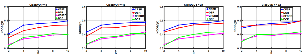
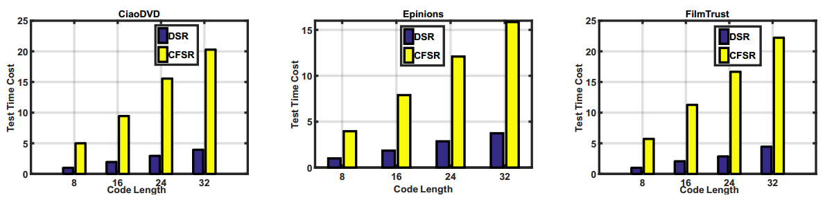
The following figures show the performance and time cost. DSR is the proposed model and r is code length.
A Unified Framework of Representation Learning and Matching Function Learning in Recommender System
Problem: Traditional recommendation problem.
Gap: Divide traditional methods into two types. One is representation learning based like MF and the other is matching function learning based like NCF. The authors combine these two kinds of methods.
Method:
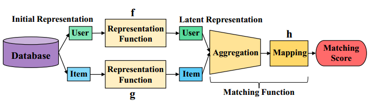
In my view, the method is under NCF framework. However, different from NCF, the representation of users and items are not randomly initialized but learning by two representation function $f$ and $g$ from raw ratings.
The method is simple. But the difficult point is to train a deep network with sparse ratings in which the model is easy to be overfitting.
An Integral Tag Recommendation Model for Textual Content
Problem: Tag recommendation
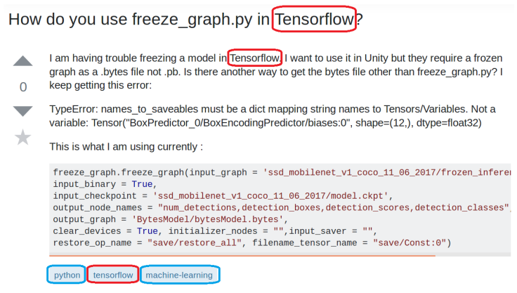
Gap: An example of tags to a text is shown in the following graph. The authors emphasize three aspects of tag recommendation that impact the accuracy: 1) sequential text modeling. This a common aspect. 2) tag correlation. The tags for a text are usually related with each other. 3) content-tag overlapping. Tags are often overlapped with the word in original text. However, there lacks an integral method that captures all the three aspects with a coherent model.
Method:
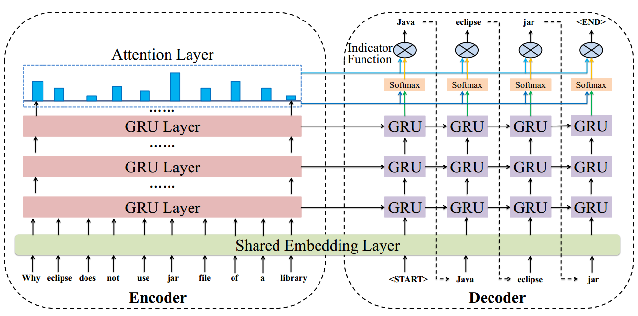
As shown in the above figure, the authors use an Multi-Layer GRU as an Encoder to encode the original text and another Multi-layer GRU as a Decoder to generate tags.
GRU could capture the order info in text
During decoding process, the previous output tag is used as the input to predict next tag. In this way, the network could capture tag correlation info.
Use a shared embedding layer to learn representation of text and tags in the same space. Besides, the author add an Indicator Function to explicitly indicate the probability of directly copying a word from the content as the tag. The probability of copying a word is calculate as
$$
o_i = v_2^T. \tanh (W_3.s_i) \
p_i = \sigma(o_i)
$$
where $s_i$ is the overall content representation for predicting current tag. $v_2$ and $W_3$ are parameters.Finally, the probability of a tag a is combination of probability of recommending a new tag and copying a word.
$$
P^{‘}(z_i) = (1-p_i)(p(z_i)) + p_i . \alpha(z_i)
$$
where $\alpha(z_i)$ is the attention weight of each word in the original text.
Hashtag Recommendation for Photo Sharing Services
Problem: Hashtag recommendation for photo sharing services
Gap: In this scenario, each photo post has a text description and each user has some historical posts with tags. So previous methods failed to capture all of image info, text info and personalized user habits in an integral model.
Method:
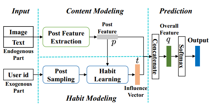
As shown in above figure, the general process is summarized as follows:
- Use a co-attention based Post Feature Extraction that considers the co-influence of image and text to extract Post Feature.
- Use Post Feature $p$ as attention point to extract representation of related tags in a user’s historical post, denoted as Influence Vector $t$
- Concatenate content feature $p$ and personal habit $t$ as the Overall Feature to give the final prediction.
Again, A Nice Attention Introduction: https://lilianweng.github.io/lil-log/2018/06/24/attention-attention.html
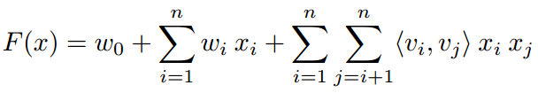
Holographic Factorization Machines for Recommendation
Problem: Recommendation basic methods
Gap: A new Holographic Factorization Machines based on FM utilizing the power of Holographic Reduced Representation.
Method: In a simply word, the authors use circular convolution operator to replace the inner product operator in FM.
FM:
HFM:
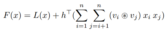
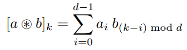
where $L(x) = w_0 + \sum_{i=1}^nw_ix_i$ and circular convolution operator(here $a$ and $b$ are both vectors other than matrix in CNN) is defined as
Evaluating Recommender System Stability with Influence-Guided Fuzzing
Problem: Evaluate the stability of Recommender System
Gap: A new aspect. The idea is similar to adversary examples in CV, but the problem is proposed independently in the paper. The authors design a method (Influence-Guided Fuzzing) to find small sets of modifications (add, remove, change) to train data that cause significantly instability of some recommendation methods.
Method: Influence-Guided Fuzzing
Inferring Influence: The authors define four kinds of influence to measure the impact of user, item, attribute and rating on recommendations.
Based on the influence defined above, the author defines some modifications to the dataset shown in the following table.
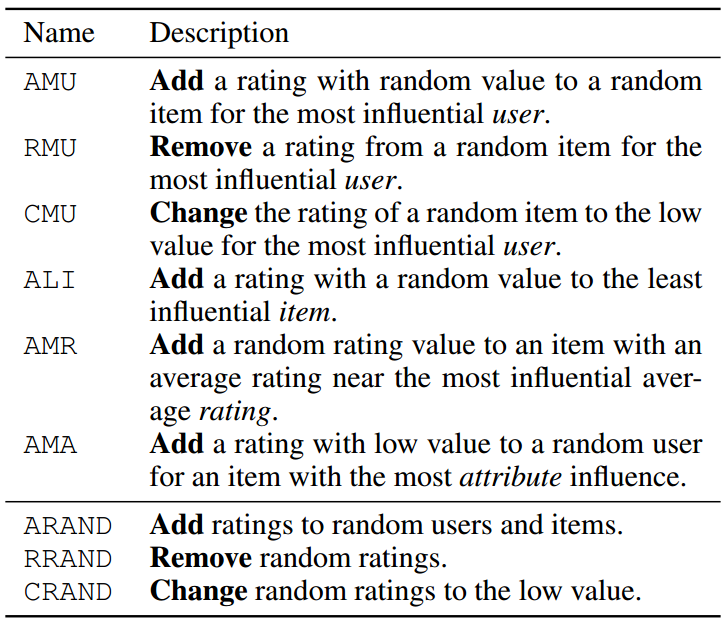
Finally, the authors apply these modifications to the dataset and test the result.
This heuristics method defines a lot modifications which are not as elegant as the gradient-based adversary examples in CV.
Joint Representation Learning for Multi-Modal Transportation Recommendation
Problem: Multi-modal transportation recommendation
Gap: Most previous works focus on improving unimodal transport planning.
Challenges to do multi-modal transportation recommendation:
- transport heterogeneity
- incomplete and implicit feedbacks
- geo-spatial locality
Method:
![]()
Firstly, a lot of work is to format data. As shown in the above figure, the authors build a MMTG (Multi-modal Transportation Graph) from all kinds of raw data. An example of MMTG is shown in the following figure.
![]()
Three kinds of nodes: Users, Transport modes, OD(Origin-Destination) pairs.
Four kinds of edges: user-user, user-mode, mode-od, od-od
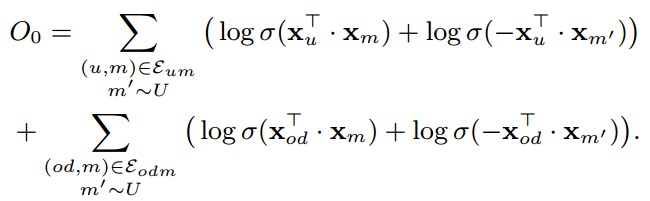
Then the personalized recommendation task is formulated as:
The data is a set of historical travel event, denote as $<u,m,od>$ where $u, m, od$ are user, mode and OD pair. Then given a new $<u, od>$, we want to recommend a most appropriate mode $m$.
Logistic loss with negative sampling
The method is simple and the contribution is to format the complex problem.
Hierarchical Reinforcement Learning for Course Recommendation in MOOCs
Problem: Course Recommendation in MOOCs
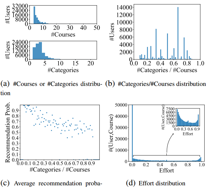
Gap: For previous attention-based works, when a user has interests in many different courses, the attention mechanism will perform poorly as the effects of the contributing courses are diluted by diverse historical courses. An example is shown in the following figure, for a trained attention-based model, the real target course get lower recommendation probability than a random selected course although it give more related courses more weights.
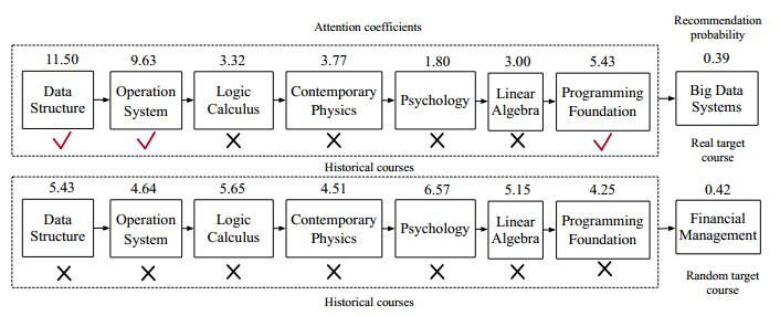
More analyses on dataset is shown in the following figure. From figure (b), we can the category ratio is evenly distributed for all users. From figure (c), we can see as the category ratio grows larger which means these users like more kinds of courses, a trained attention-based model give lower recommendation probability to the target courses.
Method: Use RL to revise user profiles by removing the noisy courses instead of assigning an attention weight to each of them.
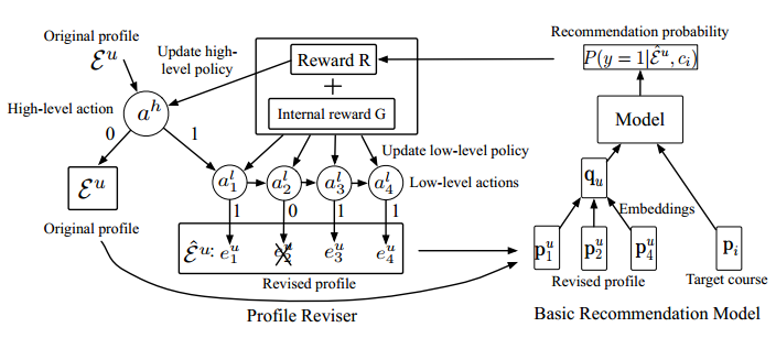
As shown in the above figure, the process is briefly summarized as:
- Use a two level Markov Decision Process(MDP) to decide how to revise the original profile. Firstly, a high level MDP to decide whether to revise the profile. Then if the high level MDP decides to revise the profile, a low level MDP will decide how to revise the profile. Finally the revised profile (maybe no change) will delivered to a basic recommendation model for training.
- The reward R to decide how to revise current profile is the difference of recommendation probabilities using revised profile and original profile. The internal reward G is the difference of similarity between (revised profile, target course) and similarity between (original profile, target course)
Other details is omitted here.
Non-Compensatory Psychological Models for Recommender Systems
Problem: Basic recommendation method
Gap: A novel aspect. The study of consumer psychology reveals two categories of consumption decision procedures: compensatory rules and non-compensatory rules. Under compensatory rules a consumer evaluates an item over all relevant aspects and a good performance on one aspect of an item compensates for poor performances on other aspects. So all traditional latent factor based methods fall into the category of compensatory rules. However, in the study of human choice behavior, it is well regarded that consumers more frequently make consumption related choice based on non-compensatory rules which do not allow the shortcomings of a product be balanced out by its attractive features. So the authors propose a method based on non-compensatory rules.
Method:
Introduction of some non-compensatory rules:
- Lexicographic rule: this rules assumes that aspects of products can be ordered in terms of importance and alternative brands are evaluated sequentially from the most prominent to the least prominent aspects.
- Conjunctive rule: This rule establishes a minimally acceptable the acceptable threshold for each aspect.
Model framework:
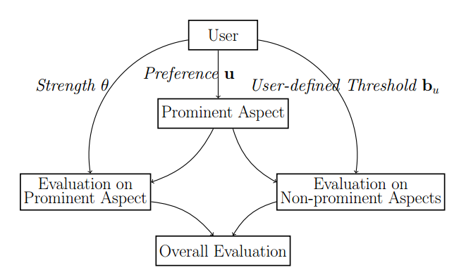
As shown in above figure, the authors assume a user’s preference on all aspects consists of two parts: prominent aspect and non-prominent part. For evaluation on prominent aspect, the score should be maximized while for evaluation on non-prominent aspects, the scores just need to satisfy some thresholds.
Following this idea, the authors changes many traditional models like MF, AMF, Local Low-rank MF, BPR. Here we take MF for an example to illustrate the work.
For traditional MF, the predicted score $\hat{X}{u,q}$ for user vector $u$ and item vector (v) is calculated as:
$$
\hat{X}{u,q} = \sum_{k=1}^Kq_ku_k
$$
where $K$ is dimension of latent factors.
Then under non-prominent rules, preference $u$ represents the a distribution of whether each aspect is a prominent aspect or not. Then for MF, the author firstly sample a prominent aspect from u as:
$$
k \sim \frac{\exp u_k}{\sum_{k^{‘}}\exp u_{k^{‘}}}
$$
Then the prominent aspect is magnified by parameter $\exp \theta$ and the non-prominent aspect should satisfy a threshold $b_{u,k^{‘}}$. Finally, the overall evaluation score is calculated as:
$$
\hat{X}{u,q} = \sum{k=1}^K\frac{\exp u_K}{\sum_{k^{‘}}\exp u_{k^{‘}}}[q_k\exp\theta + \sum_{k^{‘} \neq k}(q_{k^{‘}} - b_{u,k^{‘}})]
$$
Modeling Influential Contexts with Heterogeneous Relations for Sparse and Cold-Start Recommendation
Problem: Recommendation with influential contexts(social relation and item-item relation)
Gap:
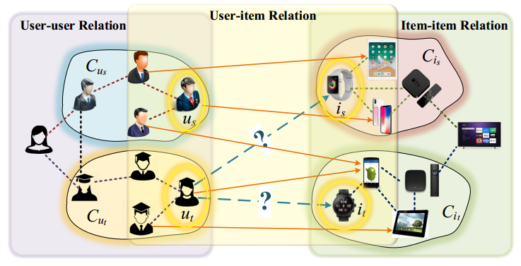
As shown in above figure, the authors format a general recommendation with influential contexts(social relation and item-item relation) and user-item interaction. In this view, most previous works have only partially considered this problem with info of at most two relations.
Method:
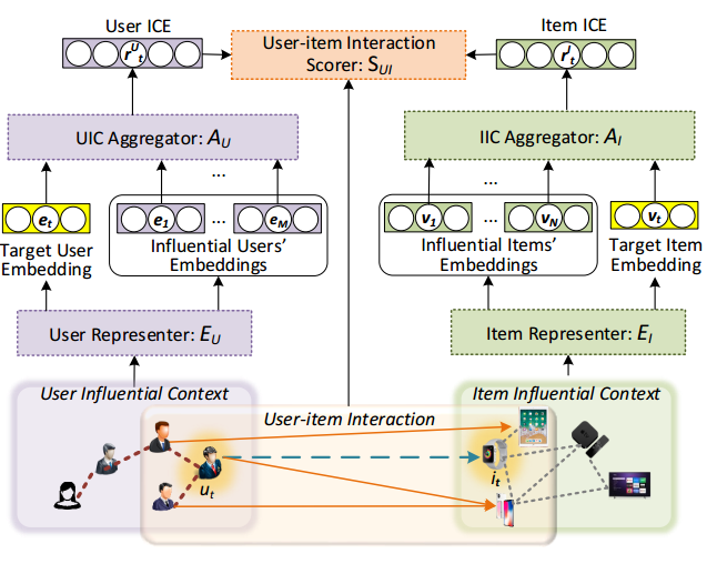
The general process is clearly shown in the above figure. The Representers $E$ is just latent embedding. The Aggregator of user has two level of modules based attention(capturing influence of friends’ friends). The Aggregator of item has only one level attention network. Finally, the User-item Interaction is inner product.
In this way, the final score contains influence of four parts as follows:

where in order the influence of four parts are: user - item, user - item context, user context - item, user context - item context.
Large-scale Interactive Recommendation with Tree-structured Policy Gradient
Problem: Interactive Recommendation (here the definition is more similar to online recommendation)
Gap: With a large number of items, traditional RL methods that handle the problem with linear time complexity is not efficient enough.
Method: Tree-structed Policy Gradient.
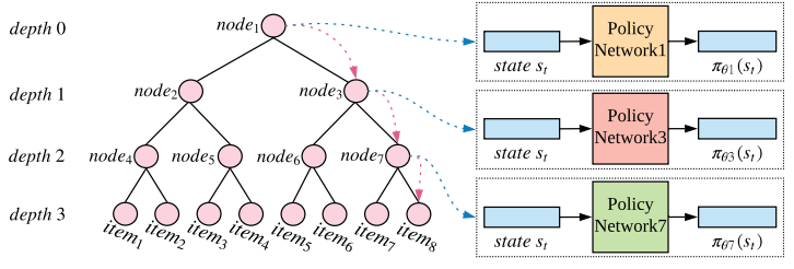
As shown in the above figure, the authors build a tree of items according to similarities of different items. Then the decision process of choosing a item is finding a path on the tree(about logN complexity) instead of finding one item from all items(N complexity)
Complexity of finding a path on the tree:
The depth of the tree is denoted as d, and each node has at most c children. Then the complexity of making decision in each Policy Network is as most c. Then total complexity is d*c which is approximately equal to logN.
The performance of this method highly depend on the quality of the built tree. The authors use three ways to represent each item as an vector and then user clustering method to cluster all items level by level to build the tree.
- Raw rating vector.
- latent factors of MF
- Use VAE to encode raw rating vector.
My concern is all these three ways are hard to learn a good representation with sparse ratings.