Assignment 3: classifiers
1 Task description
- Based on the MNIST dataset, design and implement a proper convolutional neural network.
- Based on the MNIST dataset, design and implement classifiers including: least squares with regularization, Fisher discriminant analysis (with kernels), Perceptron (with kernels), logistic regression, SVM (with kernels), MLP-NN with two different error functions.
- (optional)Based on CNN classifiers, please implement an object detection task (including face recognition).
- Design and implement a proper recurrent neural network based on LSTM or/and GRU for Sentiment Analysis. Data is available at http://deeplearning.net/tutorial/lstm.html
2 CNN on MNIST dataset
2.1 Introction to CNN(take Lenet-5 as an example)
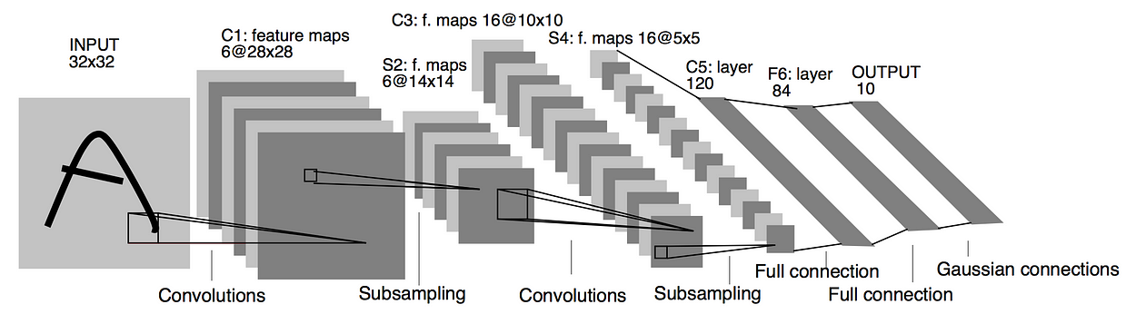
As shown in the following figure, LetNet-5 consists of three different kind of operations: convolution, pooling and full connection layer. The full connection layer was introduced in assignment 2 and will be introduce MLP part later. So here we take a look at what are convolution and pooling operation at first.
2.2 Convolution Layer
In Mathematics, for discrete variables, Convolution function is defined as follows: \begin{equation} (I \ast K)_{ij} = \sum_{m = 0}^{k_1 - 1} \sum_{n = 0}^{k_2 - 1} I(m, n)K(i-m,j-n) \end{equation} Convolution is commutative, meaning that we can equivalently write: \begin{equation} \begin{split} (I \ast K)_{ij} &= \sum_{m = 0}^{k_1 - 1} \sum_{n = 0}^{k_2 - 1} I(i-m, j-n)K(m,n) \\ &= \sum_{m = 0}^{k_1 - 1} \sum_{n = 0}^{k_2 - 1} I(i+m, j+n)K(-m,-n) \end{split} \end{equation} Usually, the latter format is more straightforward to implement in a machine learning model. We substitute kernel $K(-m,-n)$ with a flipped kernel $K(m,n)$, then we get the cross correlation function: \begin{equation} (I \otimes K)_{ij} = \sum_{m = 0}^{k_1 - 1} \sum_{n = 0}^{k_2 - 1} I(i+m, j+n)K(m,n) \end{equation} Because in CNN, kernel function K is a matrix with parameters to be trained, the cross correlation function could get the same result as convolution function with a flipped kernel matrix K. For cross correlation function is more straightforward to implement, we use it implement convolution layer in CNN.
In the case of images, we could have as input an image with height $H$, width $W$ and $C=3$ channels (red, blue and green) such that $I\in R^{H×W×C}$. The number of output channels id $D$. Subsequently for a bank of $D$ filters, we have $K \in R^{k_1×k_2×C×D}$ and biases $b \in R^D$, one for each filter. The output from this convolution procedure is as follows: \begin{equation} (I \ast K_d)_{ij} = \sum_{m = 0}^{k_1 - 1} \sum_{n = 0}^{k_2 - 1} \sum_{c = 1}^{C} K_{m,n,c,d} \cdot I_{i+m, j+n, c} + b_d \end{equation} We denote the activation function as $a(.)$, the activation of the l-th convolution layer as $x_{ij}^l$, and the output vector of the l-th convolution layer as $o^{l}$, then, \begin{equation} x_{ijd}^1 = (I \ast K_d)_{ij} \end{equation} \begin{equation} o_{ijd}^{1} = a(x_{ijd}^1) \end{equation} The following convolution layer is just the same as the first with the input being the output of in the previous layer.
2.3 Pooling layer
In LeNet-5, there is a (max) pooling layer each convolution layer. At the pooling layer, forward propagation results in an $N \times N$ pooling block being reduce to a single value. For Max-pooling, the value is the biggest value in the pooling block. For Average pooling, the value is the average of all values in the pooling block. We denote the output of l-th pooling layer as $p^l$, then take max-pooling for an example, we get \begin{equation} p^l_{ijd} = \max\{o_{mnd}^l|i \le m < i + N, j \le n < j + N\} \end{equation} For average pooling, we just need substitute operation $max$ with operation $avg$ which mean get the average of the all values in the set.
2.4 Back propagation for each kind of layer (refer to new post for correct solutions)
Convolution between the input feature map of dimension $H×W$ with C channels and the weight kernel of dimension $k_1×k_2$ produces an output feature map of size $(H−k_1+1) \times (W−k_2+1)$. The number of input channels and output channels are $C$ and $D$. The gradient component for the individual weights can be obtained by applying the chain rule in the following way: \begin{equation} \begin{split} \frac{\partial L(t,y)}{\partial w_{m^{\prime},n^{\prime},c,d}^l} &= \sum_{i=0}^{H-k_1} \sum_{j=0}^{W-k_2} \frac{\partial L(t,y)}{\partial x_{i,j,d}^{l}} \frac{\partial x_{i,j,d}^{l}}{\partial w_{m^{\prime},n^{\prime},c,d}^l} \\ &= \sum_{i=0}^{H-k_1} \sum_{j=0}^{W-k_2} \delta^{l}_{i,j,d} \frac{\partial x_{i,j,d}^{l}}{\partial w_{m^{\prime},n^{\prime},c,d}^l} \\ &= \sum_{i=0}^{H-k_1} \sum_{j=0}^{W-k_2} \delta^{l}_{i,j,d} \frac{\partial}{\partial w_{m^{\prime},n^{\prime},c,d}^l}\left( \sum_{m} \sum_{n} \sum_{c=1}^C w_{m,n,c,d}^{l}o_{i+m, j+n,c}^{l-1} + b^l_d \right) \\ &= \sum_{i=0}^{H-k_1} \sum_{j=0}^{W-k_2} \delta^{l}_{i,j,c} \frac{\partial}{\partial w_{m^{\prime},n^{\prime},c,d}^l}\left( w_{m^{\prime},n^{\prime},c,d}^{l} o_{ i + m^{\prime}, j + n^{\prime},c}^{l-1}\right) \\ &= \sum_{i=0}^{H-k_1} \sum_{j=0}^{W-k_2} \delta^{l}_{i,j,c} o_{i+m^{\prime},j+n^{\prime},c}^{l-1} \end{split} \end{equation} \begin{equation} \begin{split} \frac{\partial L(t,y)}{\partial b^l_d} &= \sum_{i=0}^{H-k_1} \sum_{j=0}^{W-k_2} \frac{\partial L(t,y)}{\partial x_{i,j,d}^{l}} \frac{\partial x_{i,j,d}^{l}}{\partial b^l_d} \\ &= \sum_{i=0}^{H-k_1} \sum_{j=0}^{W-k_2} \delta^{l}_{i,j,d} \frac{\partial x_{i,j,d}^{l}}{\partial b^l_d} \\ &= \sum_{i=0}^{H-k_1} \sum_{j=0}^{W-k_2} \delta^{l}_{i,j,d} \frac{\partial}{\partial b^l_d}\left( \sum_{m} \sum_{n} \sum_{c=1}^C w_{m,n,c,d}^{l}o_{i+m, j+n,c}^{l-1} + b^l_d \right) \\ &= \sum_{i=0}^{H-k_1} \sum_{j=0}^{W-k_2} \delta^{l}_{i,j,d} \end{split} \end{equation} where we denote $\frac{\partial L(t,y)}{\partial x_{i,j,d}^{l}}$ as $\delta^{l}_{i,j,d}$ that represents the error in layer $l$.
There is no parameter in pooling layer. And the Gradient rooting is done in the following ways.
- Max-pooling - the error is just assigned to where it comes from - the “winning unit” because other units in the previous layer’s pooling blocks did not contribute to it hence all the other assigned values of zero
- Average pooling - the error is multiplied by 1/N×N and assigned to the whole pooling block (all units get this same value).
2.5 Back propagation in LeNet-5
LeNet-5 includes full connection layer, pooling layer and convolution layer. Using chain rule and gradients in section 2 and 3.3, we can easily get the gradients of all parameters in LeNet-5.
2.6 Implementation and experiments on MNSIT
import tensorflow as tf
def cnn_initializer(image_width=28, image_height=28, class_num=10):
    def cnn_model_fn(features, labels, mode):
      """Model function for CNN."""
      # Input Layer
      input_layer = tf.reshape(features["x"], [-1, image_width, image_height, 1])

      # Convolutional Layer #1
      conv1 = tf.layers.conv2d(
          inputs=input_layer,
          filters=32,
          kernel_size=[5, 5],
          padding="same",
          activation=tf.nn.relu)

      # Pooling Layer #1
      pool1 = tf.layers.max_pooling2d(inputs=conv1, pool_size=[2, 2], strides=2)

      # Convolutional Layer #2 and Pooling Layer #2
      conv2 = tf.layers.conv2d(
          inputs=pool1,
          filters=64,
          kernel_size=[5, 5],
          padding="same",
          activation=tf.nn.relu)
      pool2 = tf.layers.max_pooling2d(inputs=conv2, pool_size=[2, 2], strides=2)

      # Dense Layer
      pool2_flat = tf.reshape(pool2, [-1, image_width * image_height * 64 / 16])
      dense = tf.layers.dense(inputs=pool2_flat, units=1024, activation=tf.nn.relu)

      # we add advanced dropout layer that is not involed in LeNet-5
      dropout = tf.layers.dropout(
          inputs=dense, rate=0.4, training=mode == tf.estimator.ModeKeys.TRAIN)

      # Logits Layer
      logits = tf.layers.dense(inputs=dropout, units=class_num)

      predictions = {
          # Generate predictions (for PREDICT and EVAL mode)
          "classes": tf.argmax(input=logits, axis=1),
          # Add `softmax_tensor` to the graph. It is used for PREDICT and by the
          # `logging_hook`.
          "probabilities": tf.nn.softmax(logits, name="softmax_tensor")
      }

      if mode == tf.estimator.ModeKeys.PREDICT:
        return tf.estimator.EstimatorSpec(mode=mode, predictions=predictions)

      # Calculate Loss (for both TRAIN and EVAL modes)
      loss = tf.losses.sparse_softmax_cross_entropy(labels=labels, logits=logits)

      # Configure the Training Op (for TRAIN mode)
      if mode == tf.estimator.ModeKeys.TRAIN:
        optimizer = tf.train.GradientDescentOptimizer(learning_rate=0.001)
        train_op = optimizer.minimize(
            loss=loss,
            global_step=tf.train.get_global_step())
        return tf.estimator.EstimatorSpec(mode=mode, loss=loss, train_op=train_op)

      # Add evaluation metrics (for EVAL mode)
      eval_metric_ops = {
          "accuracy": tf.metrics.accuracy(
              labels=labels, predictions=predictions["classes"])}
      return tf.estimator.EstimatorSpec(
          mode=mode, loss=loss, eval_metric_ops=eval_metric_ops)
    return cnn_model_fn
# load data
import numpy as np
# Load training and eval data
mnist = tf.contrib.learn.datasets.load_dataset("mnist")
train_data = mnist.train.images  # Returns np.array
train_labels = np.asarray(mnist.train.labels, dtype=np.int32)
eval_data = mnist.test.images  # Returns np.array
eval_labels = np.asarray(mnist.test.labels, dtype=np.int32)
def main():
    config = tf.estimator.RunConfig(log_step_count_steps=10000)
    # Create the Estimator
    mnist_classifier = tf.estimator.Estimator(
        model_fn=cnn_initializer(), config=config, model_dir="./tmp/mnist_convnet_model")

    # Train the model
    train_input_fn = tf.estimator.inputs.numpy_input_fn(
        x={"x": train_data},
        y=train_labels,
        batch_size=100,
        num_epochs=None,
        shuffle=True)
    mnist_classifier.train(
        input_fn=train_input_fn,
        steps=20000)
    # Evaluate the model and print results
    eval_input_fn = tf.estimator.inputs.numpy_input_fn(
        x={"x": eval_data},
        y=eval_labels,
        num_epochs=1,
        shuffle=False)
    eval_results = mnist_classifier.evaluate(input_fn=eval_input_fn)
    print(eval_results)

# run model
main()
# store the accuracy
all_accuracy = {}
all_accuracy['CNN'] = 0.9712
The final accuracy on MNIST test set is 0.9712. The loss curve over train steps is as follows:

3 Other classifiers
3.1 Least squares with regularization for classfication
The simplest linear model for regression is one that involves a linear combination of the input variables. Here, we donate input variables or features as $x = (x_1, ..., x_D)^T$ and then the target output is calculated as follows: $$ y(x,w) = w_0 + w_1x_1 + ... + w_dx_D $$
Obviously, this imposes significant limitations on the model. For example, the model can not fit a ploynomial curve with input x being a scalar. We therefore extend the model by considering linear combinations of fixed nonlinear functions of the input variables, of the form $$ y(x,w) = w_0 + \sum_{j=1}^{M-1}w_j\phi_j(x)$$
where $\phi_j(x)$ are known as basic functions. In boston house price predicting problem, the input x is a 13 dimension vector. So we can simply define $\phi_j(x) = x_j$. On the other hand, in UK house price predicting problem, the input x is just a scalar. This is a polinomial curve fitting problem. So we can define $\phi_j(x) = x^j$ and then the curve could be well fitted by the polynomial function.
Besides, We can define $\phi_0(x) = 1$ so that $$y(x,w) = \sum_{j=0}^{M-1}w_j\phi_j(x) = w^T\phi(x)$$
Then,Basic Linear Regression estimates the parameters by minimizing the residual sum of squares between the observed responses, donated as t, in the dataset and the responses($y(x,w)$) predicted by the linear approximation. Mathematically linear regression with regularization solves a problem of the form: $$ \min_{w} {{|| y(x,w) - t||_2}^2 + \alpha {||w||_2}^2} $$ Here, $\alpha \geq 0$ is a complexity parameter that controls the amount of shrinkage: the larger the value of , the greater the amount of shrinkage and thus the coefficients become more robust to collinearity.
Obviously, we can use this model to do classification task by simply denote the label as a 1-of-K binary coding vector t. And each class $C_k$ is described by its own linear model so that $$ y_k(x,w_k) = w_k^T \phi(x) $$ , then the loss function will be $$ l(y,t) = \frac{1}{K}\sum_k {{|| y(x,w_k) - t_k||_2}^2 + \alpha {||w_k||_2}^2} $$ Then, we choose the index of bigget y_k as the target label.Here we use sklearn to implement this model as follows.
from sklearn.linear_model import RidgeClassifier
def accuracy_fn(preds, labels):
    return np.mean(np.equal(labels, preds).astype(np.float32))
def train_and_test_model(model):
    model.fit(train_data, train_labels)
    preds = model.predict(eval_data)
    return accuracy_fn(preds, eval_labels)
all_accuracy['RidgeClassifier'] = train_and_test_model(RidgeClassifier())
print('accuracy of Ridge classifier: {:.4f}'.format(all_accuracy['RidgeClassifier']))
3.2 Fisher discriminant analysis (with kernels)
Fisher discriminant analysis is also known as linear discriminant analysis(LDA). One way to explain LDA is in terms of dimensionality reduction. For input vector x, we project it into one diamension using $$ y = w^Tx $$ For two classes $C_1$ and $C_2$, the mean vectors of the two classes are given by $$ m_1 = \frac{1}{N_1}\sum_{n \in C_1}x_n \\ m_2 = \frac{1}{N_2}\sum_{n \in C_2}x_n $$ Then we project mean vectors $m_1$ and $m_2$ in to one diamension scalar $y_1$ and $y_2$. The target of LDA is to maximize $$ (y_2 - y_1)^2 = W^TS_BW \\ S_B = (m_2 - m_1)(m_2 - m_1)^T $$ where $S_B$ is known as between-class covariance.
Besides the within-class of the transformed data in $C_k$ is given by $$ s_k^2 = \sum_{C_k}(y_n -m_k)^2 $$ And LDA also needs to minimize $s_1^2 + s_2^2 = w^TS_Ww$ where $S_w$ is within-class covariance matrix, given by $$ S_w = \sum_{n \in C_1}(x_n -m_1)(x_n - m_1)^T + \sum_{n \in C_2}(x_n -m_2)(x_n - m_2)^T $$ The final loss of LDA is $$ J(w) = \frac{w^TS_Bw}{w^TS_Ww} $$
To extend LDA to non-linear mappings, the data, given as the $ \ell$ points ${\displaystyle \mathbf {x} _{i},} $ can be mapped to a new feature space, ${\displaystyle F,}$ via some function $ \phi$ . In this new feature space, the function that needs to be maximized is
$${\displaystyle J(\mathbf {w} )={\frac {\mathbf {w} ^{\text{T}}\mathbf {S} _{B}^{\phi }\mathbf {w} }{\mathbf {w} ^{\text{T}}\mathbf {S} _{W}^{\phi }\mathbf {w} }},}$$where
$${\displaystyle {\begin{aligned}\mathbf {S} _{B}^{\phi }&=\left(\mathbf {m} _{2}^{\phi }-\mathbf {m} _{1}^{\phi }\right)\left(\mathbf {m} _{2}^{\phi }-\mathbf {m} _{1}^{\phi }\right)^{\text{T}}\\\mathbf {S} _{W}^{\phi }&=\sum _{i=1,2}\sum _{n=1}^{l_{i}}\left(\phi (\mathbf {x} _{n}^{i})-\mathbf {m} _{i}^{\phi }\right)\left(\phi (\mathbf {x} _{n}^{i})-\mathbf {m} _{i}^{\phi }\right)^{\text{T}},\end{aligned}}} $$and
$${\displaystyle \mathbf {m} _{i}^{\phi }={\frac {1}{l_{i}}}\sum _{j=1}^{l_{i}}\phi (\mathbf {x} _{j}^{i}).} $$See Multi-class_KFD for KFD for multiclass classification. Here we use sklearn lib to implement the model.
from sklearn.discriminant_analysis import LinearDiscriminantAnalysis
all_accuracy['LDA'] = train_and_test_model(LinearDiscriminantAnalysis())
print('accuracy of linear discriminant analysis: {:.4f}'.format(all_accuracy['LDA']))
3.3 Perceptron
For the perceptron algorithm, it is more convenient to use the target values of $t = +1$ for class $C_1$ and $t = -1$ for class $C_1$. Using the $ t \in \{-1, +1\}$ target coding scheme it follows that we would like all patterns to satisfy $w^T\phi(x_n)t_n > 0$. So error funtionc the perceptron is therefore given by $$ E_p(x) = -\sum_{n \in M} w^T \phi_nt_n $$ See Multiclass_perceptron for perceptron algrithm for multi-class classification.
from sklearn.linear_model import Perceptron
all_accuracy['Perceptron'] = train_and_test_model(Perceptron())
print('accuracy of Perceptron: {:.4f}'.format(all_accuracy['Perceptron']))
3.4 Logistic regression
As the same as the above, we begin our treatment of the generalized linear models by considering the problem of two-class classification. Logistic regression is a probabilitic model. The posterior probability of class $C_1$ can be written as a logitic sigmoid acting on a linear function of the feature vector $\phi$ so that $$ p(C_1|\phi) = y(\phi) = \sigma(w^T\phi) $$ with $p(C_2|\phi) = 1 - p(C_1|\phi)$. Here $\sigma(.)$ is the logistic sigmoid function defined as $$ \sigma(x) = \frac{1}{1 + \exp(-x)} $$
For a training data set $\{\phi_n, t_n\}$, with $n = 1, 2, ..., N$, the likelihood function can be written as $$ p(t|w) = \prod_{n=1}^N y_n^{t^n}(1 - y_n)^{1 - t_n} $$ where $t = (t_1, ..., t_N)$ and $y_n = p(C_1|\phi_n)$. Then we can define the error funtion be the negtive log likelihood function. $$ E(w) = -lnp(t|w) = - \sum_{n=1}^N (t_nlny_n + (1 - t_nln(1 - y_n)) $$
For multiclass classification, we can define the posterior probability as the softmax transformation of the linear function fo the feature variables, so that $$ p(C_k|\phi) = y_k(\phi) = \frac{exp(w_k^T\phi)}{\sum_jexp(w_j^T\phi} $$ The likelihood function is then given by $$ p(T|w_1,..,w_K) = \prod_{n=1}^N\prod_{k=1}^K p(C_k|\phi_n)^{t_{nk}} = \prod_{n=1}^N\prod_{k=1}^K y_{nk}^{t_{nk}} $$
Thake the negtive logarithm as the error function, then we get $$ E(W) = -ln p(T|w_1,..,w_K) = -\sum_{n=1}^N\sum_{k=1}^K {t_{nk}}ln y_{nk} $$
from sklearn.linear_model import LogisticRegression

all_accuracy['LogisticRegression'] = train_and_test_model(LogisticRegression())
print('accuracy of LogisticRegression: {:.4f}'.format(all_accuracy['LogisticRegression']))
3.4 SVM with kernels
SVM is also known as larger margin classifer which usually has a smaller generalization error. When a SVM classifier is trained, only the data points that are nearest to decision boundary are left for classify a new data point. These remaining data points called support vectors.
For detail intuition and processm, see PRML book chapter 7. Here we briefy introduce the taget.
Given training vectors $x_i \in \mathbb{R}^p$, i=1,…, n, in two classes, and a vector $y \in \{1, -1\}^n$, SVC solves the following primal problem: $$ \begin{align}\begin{aligned}\min_ {w, b, \zeta} \frac{1}{2} w^T w + C \sum_{i=1}^{n} \zeta_i\\\begin{split}\textrm {subject to } & y_i (w^T \phi (x_i) + b) \geq 1 - \zeta_i,\\ & \zeta_i \geq 0, i=1, ..., n\end{split}\end{aligned}\end{align} $$
Its dual is $$ \begin{align}\begin{aligned}\min_{\alpha} \frac{1}{2} \alpha^T Q \alpha - e^T \alpha\\\begin{split} \textrm {subject to } & y^T \alpha = 0\\ & 0 \leq \alpha_i \leq C, i=1, ..., n\end{split}\end{aligned}\end{align} $$
where $e$ is the vector of all ones, $C > 0$ is the upper bound, $Q$ is an $n$ by $n$ positive semidefinite matrix, $Q_{ij} \equiv y_i y_j K(x_i, x_j)$ , where $K(x_i, x_j) = \phi (x_i)^T \phi (x_j)$ is the kernel. Here training vectors are implicitly mapped into a higher (maybe infinite) dimensional space by the function .
The decision function is: $$ \operatorname{sgn}(\sum_{i=1}^n y_i \alpha_i K(x_i, x) + \rho) $$
The common used kernel function can be any of the following:
linear: $\langle x, x'\rangle $.
polynomial: $(\gamma \langle x, x'\rangle + r)^d$.
rbf: $\exp(-\gamma \|x-x'\|^2)$
sigmoid (\tanh(\gamma \langle x,x'\rangle + r))
from sklearn.svm import SVC

all_accuracy['SVC'] = train_and_test_model(SVC(kernel='linear'))
print('accuracy of SVC: {:.4f}'.format(all_accuracy['SVC']))
3.5 MLP-NN with two different error functions
3.5.1 Forward propagation
 As shown in the Figure, we denote input layer as $x$ and $x_k$ represents the value of the k-th unit of input layer. we denote $a(.)$ as the activation function, $o^{(1)}$ as the activation of the hidden layer, and $\{W^{(1)}, b^{(1)}\}$ as the weights and bias from input layer to hidden layer, then the hidden layer, denoted as $h$, is calculated as follows:
\begin{equation}
o^{(1)} = W^{(1)}x + b^{(1)}
\end{equation}
\begin{equation}
h = a(o^{(1)})
\end{equation}
As the same as above, we denote output layer as a vector $y$, the activation as $o^{(2)}$, and the weights and bias from hidden layer to output layer as $\{W^{(2)}, b^{(2)}\}$, then the output vector is calculated as follows:
\begin{equation}
o^{(2)} = W^{(2)}h + b^{(2)}
\end{equation}
\begin{equation}
y = a(o^{(2)})
\end{equation}
Finally, we denote the true target value as a vector $t$ and the error function as $L(t, y)$.
As shown in the Figure, we denote input layer as $x$ and $x_k$ represents the value of the k-th unit of input layer. we denote $a(.)$ as the activation function, $o^{(1)}$ as the activation of the hidden layer, and $\{W^{(1)}, b^{(1)}\}$ as the weights and bias from input layer to hidden layer, then the hidden layer, denoted as $h$, is calculated as follows:
\begin{equation}
o^{(1)} = W^{(1)}x + b^{(1)}
\end{equation}
\begin{equation}
h = a(o^{(1)})
\end{equation}
As the same as above, we denote output layer as a vector $y$, the activation as $o^{(2)}$, and the weights and bias from hidden layer to output layer as $\{W^{(2)}, b^{(2)}\}$, then the output vector is calculated as follows:
\begin{equation}
o^{(2)} = W^{(2)}h + b^{(2)}
\end{equation}
\begin{equation}
y = a(o^{(2)})
\end{equation}
Finally, we denote the true target value as a vector $t$ and the error function as $L(t, y)$.
3.5.2 General back-propagation
Then, in the back-propagation process, the gradients of each weight and bias from can be estimate using chain derivation rule as follows: \begin{equation} \begin{split} \frac{\partial L(t,y)}{\partial w^{(2)}_{ji}} &= \frac{\partial L(t,y)}{\partial y_i} \frac{\partial y_i}{\partial o_i^{(2)}} \frac{\partial o_i^{(2)}}{\partial w^{(2)}_{ji}} \\ &= \frac{\partial L(t,y)}{\partial y_i}\frac{\partial y_i}{\partial o_i^{(2)}}h_j \end{split} \end{equation} \begin{equation} \begin{split} \frac{\partial L(t,y)}{\partial b^{(2)}_{j}} &= \frac{\partial L(t,y)}{\partial y_i} \frac{\partial y_i}{\partial o_i^{(2)}} \frac{\partial o_i^{(2)}}{\partial b^{(2)}_{j}} \\ &= \frac{\partial L(t,y)}{\partial y_i}\frac{\partial y_i}{\partial o_i^{(2)}} \end{split} \end{equation} \begin{equation} \begin{split} \frac{\partial L(t,y)}{\partial w^{(1)}_{kj}} &= \sum_i\frac{\partial L(t,y)}{\partial y_i} \frac{\partial y_i}{\partial o_i^{(2)}} \frac{\partial o_i^{(2)}}{\partial h_{j}} \frac{\partial h_{j}}{\partial o_j^{(1)}} \frac{\partial o_j^{(1)}}{\partial w^{(1)}_{kj}} \\ &= \sum_i\frac{\partial L(t,y)}{\partial y_i} \frac{\partial y_i}{\partial o_i^{(2)}} w^{(2)}_{ji} \frac{\partial h_{j}}{\partial o_j^{(1)}} x_k \end{split} \end{equation} \begin{equation} \begin{split} \frac{\partial L(t,y)}{\partial b^{(1)}_{k}} &= \sum_i\frac{\partial L(t,y)}{\partial y_i} \frac{\partial y_i}{\partial o_i^{(2)}} \frac{\partial o_i^{(2)}}{\partial h_{j}} \frac{\partial h_{j}}{\partial o_j^{(1)}} \frac{\partial o_j^{(1)}}{\partial b^{(1)}_{k}} \\ &= \sum_i\frac{\partial L(t,y)}{\partial y_i} \frac{\partial y_i}{\partial o_i^{(2)}} w^{(2)}_{ji} \frac{\partial h_{j}}{\partial o_j^{(1)}} \end{split} \end{equation}
3.5.3 L2 difference loss
For the l2 difference loss function defined as follows, \begin{equation} L(t,y) = \frac{1}{2}\sum_i(t_i - y_i)^2 \end{equation} \begin{equation} \label{eq:partial_l2} \frac{\partial L(t,y)}{\partial y_i} = -(t_i - y_i) = (y_i - t_i) \end{equation} we substitute $\frac{\partial L(t,y)}{\partial y_i}$ in the equations from 5 to 8 with $(y_i - t_i)$. Then we can get \begin{equation} \frac{\partial L(t,y)}{\partial w^{(2)}_{ji}} = (y_i - t_i)\frac{\partial y_i}{\partial o_i^{(2)}}h_j \end{equation} \begin{equation} \frac{\partial L(t,y)}{\partial b^{(2)}_{j}} = (y_i - t_i)\frac{\partial y_i}{\partial o_i^{(2)}} \end{equation} \begin{equation} \frac{\partial L(t,y)}{\partial w^{(1)}_{kj}} = \sum_i (y_i - t_i) \frac{\partial y_i}{\partial o_i^{(2)}} w^{(2)}_{ji} \frac{\partial h_{j}}{\partial o_j^{(1)}} x_k \end{equation} \begin{equation} \frac{\partial L(t,y)}{\partial b^{(1)}_{k}}= \sum_i (y_i - t_i) \frac{\partial y_i}{\partial o_i^{(2)}} w^{(2)}_{ji} \frac{\partial h_{j}}{\partial o_j^{(1)}} \end{equation}
3.5.4 Cross entropy loss
For the cross entropy loss function defined as follows, \begin{equation} L(t,y) = \sum_i -t_i\log y_i \end{equation} \begin{equation} \frac{\partial L(t,y)}{\partial y_i} = -\frac{t_i}{y_i} \end{equation} we substitute $\frac{\partial L(t,y)}{\partial y_i}$ in the equations from 5 to 8 with $-\frac{t_i}{y_i}$. Then we can get \begin{equation} \frac{\partial L(t,y)}{\partial w^{(2)}_{ji}} = -\frac{t_i}{y_i}\frac{\partial y_i}{\partial o_i^{(2)}}h_j \end{equation} \begin{equation} \frac{\partial L(t,y)}{\partial b^{(2)}_{j}} = -\frac{t_i}{y_i}\frac{\partial y_i}{\partial o_i^{(2)}} \end{equation} \begin{equation} \frac{\partial L(t,y)}{\partial w^{(1)}_{kj}} = \sum_i -\frac{t_i}{y_i} \frac{\partial y_i}{\partial o_i^{(2)}} w^{(2)}_{ji} \frac{\partial h_{j}}{\partial o_j^{(1)}} x_k \end{equation} \begin{equation} \frac{\partial L(t,y)}{\partial b^{(1)}_{k}}= \sum_i -\frac{t_i}{y_i} \frac{\partial y_i}{\partial o_i^{(2)}} w^{(2)}_{ji} \frac{\partial h_{j}}{\partial o_j^{(1)}} \end{equation} In addition, cross entropy is usually to be used with softmax logits
3.5.5 Sigmoid activation function
If the activation function $a(.)$ is the sigmoid function defined as follows, \begin{equation} a(x) = \frac{1}{1 + exp^{-x}} \end{equation} \begin{equation} \frac{\partial a(x)}{\partial x} = a(x)(1-a(x)) \end{equation} then the corresponding $\frac{\partial a(x)}{\partial x}$ can be substituted with $a(x)(1-a(x))$ as the same as above.
3.5.6 Implementation and experiments
# Parameters
learning_rate = 0.01
num_steps = 1000
batch_size = 128
display_step = 200

# Network Parameters
n_hidden_1 = 256 # 1st layer number of neurons
n_hidden_2 = 256 # 2nd layer number of neurons
num_input = 784 # MNIST data input (img shape: 28*28)
num_classes = 10 # MNIST total classes (0-9 digits)
one_hot_matrix = np.eye(num_classes)
# Define the neural network
def neural_net(x):
    # Hidden fully connected layer with 256 neurons
    layer_1 = tf.layers.dense(x, n_hidden_1)
    # Hidden fully connected layer with 256 neurons
    layer_2 = tf.layers.dense(layer_1, n_hidden_2)
    # Output fully connected layer with a neuron for each class
    out_layer = tf.layers.dense(layer_2, num_classes)
    return out_layer
def train_model(loss='cross_entropy'):
    # tf Graph input
    X = tf.placeholder("float", [None, num_input])
    Y = tf.placeholder("float", [None, num_classes])

    # Construct model
    logits = neural_net(X)

    # Define loss and optimizer
    if loss == 'cross_entropy':
        loss_op = tf.reduce_mean(tf.nn.softmax_cross_entropy_with_logits(
            logits=logits, labels=Y))
    else:
        loss_op = tf.reduce_mean(tf.squared_difference(logits, Y))
    optimizer = tf.train.AdamOptimizer(learning_rate=learning_rate)
    train_op = optimizer.minimize(loss_op)

    # Evaluate model (with test logits, for dropout to be disabled)
    correct_pred = tf.equal(tf.argmax(logits, 1), tf.argmax(Y, 1))
    accuracy = tf.reduce_mean(tf.cast(correct_pred, tf.float32))

    # Initialize the variables (i.e. assign their default value)
    init = tf.global_variables_initializer()


    # Start training
    with tf.Session() as sess:

        # Run the initializer
        sess.run(init)

        for step in range(1, num_steps+1):
            batch_x, batch_y = mnist.train.next_batch(batch_size)
            batch_y = one_hot_matrix[batch_y]
            # Run optimization op (backprop)
            sess.run(train_op, feed_dict={X: batch_x, Y: batch_y})
            if step % display_step == 0 or step == 1:
                # Calculate batch loss and accuracy
                loss, acc = sess.run([loss_op, accuracy], feed_dict={X: batch_x,
                                                                     Y: batch_y})
                print("Step " + str(step) + ", Minibatch Loss= " + \
                      "{:.4f}".format(loss) + ", Training Accuracy= " + \
                      "{:.3f}".format(acc))

        print("Optimization Finished!")

        # Calculate accuracy for MNIST test images
        test_accuracy = sess.run(accuracy, feed_dict={X: mnist.test.images,
                                          Y: one_hot_matrix[mnist.test.labels]})
        print("Testing Accuracy:", test_accuracy)

        return test_accuracy
mlp_with_entropy_loss_acc = train_model()
all_accuracy['mlp_with_entropy_loss'] = mlp_with_entropy_loss_acc
mlp_with_square_loss_acc = train_model(loss='square_loss')
all_accuracy['mlp_with_square_loss'] = mlp_with_square_loss_acc
4 Performance comparison on MNIST
import pandas as pd
all_acc = {}
for key in all_accuracy:
    all_acc[key] = [all_accuracy[key]]
pd.DataFrame.from_dict(all_acc)
# we can see that CNN performs significiantly beterr than others. SVC is the second one and LR gets the third place.
5 CNN for simple face detection
5.1 build dataset
# show image demo
% matplotlib inline
import matplotlib.pyplot as plt
import os
from PIL import Image

data_dir = './data/face/yalefaces/'
for filename in os.listdir(data_dir):
    # print filename example
    print filename
    im = Image.open(data_dir + filename).resize((80,60))
    im_array = np.array(im)
    print im_array.shape
    plt.imshow(im_array, cmap='gray')
    plt.axis('off')
    break
# the format is subject{id}.{expression}

images = []
labels = []
for filename in os.listdir(data_dir):
    im = Image.open(data_dir + filename).resize((80, 60))
    images.append((np.array(im).flatten() / 255.).tolist())
    labels.append(int(filename[7:9]) - 1)
images = np.array(images)
labels = np.array(labels)
print(images.shape, labels.shape)
## build train and test set
test_p = 0.2
cut = int(len(images)*test_p)
images_train = images[: cut]
labels_train = labels[: cut]
images_test = images[cut:]
labels_test = labels[cut:]
5.2 Train Model
def main_face():
    config = tf.estimator.RunConfig(log_step_count_steps=200)
    # Create the Estimator
    mnist_classifier = tf.estimator.Estimator(
        model_fn=cnn_initializer(60, 80, 15), config=config, model_dir="./tmp/face_convnet_model")

    # Train the model
    train_input_fn = tf.estimator.inputs.numpy_input_fn(
        x={"x": images_train},
        y=labels_train,
        batch_size=10,
        num_epochs=None,
        shuffle=True)
    mnist_classifier.train(
        input_fn=train_input_fn,
        steps=1000)
    # Evaluate the model and print results
    eval_input_fn = tf.estimator.inputs.numpy_input_fn(
        x={"x": images_test},
        y=labels_test,
        num_epochs=1,
        shuffle=False)
    eval_results = mnist_classifier.evaluate(input_fn=eval_input_fn)
    print(eval_results)

# run model
main_face()
# I have tuned the hyperparameters, final accuracy on test set is 0.51. Orz
6 RNN, LSTM, GRU
Please see this great blog http://colah.github.io/posts/2015-08-Understanding-LSTMs/. I just give a summary here.
6.1 RNN
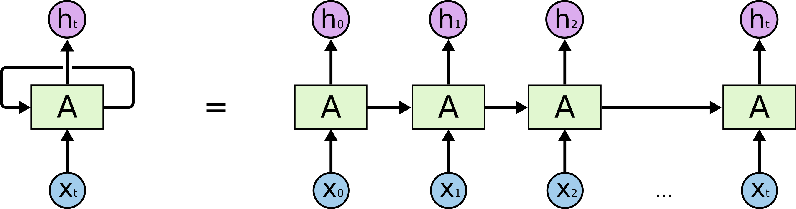 The above figure is an unrolled recurrent neural network. $h_i$ is the hidden layer at step $i$. Usually, we will add an additional layer on hidden layer $h_i$ to get the ouput at step $i$. When RNN is unrolled, we can treat it as a common multi layer network.
One of the appeals of RNNs is the idea that they might be able to connect previous information to the present task, such as using previous video frames might inform the understanding of the present frame. If RNNs could do this, they’d be extremely useful. But can they? It depends.
Sometimes, we only need to look at recent information to perform the present task. For example, consider a language model trying to predict the next word based on the previous ones. If we are trying to predict the last word in “the clouds are in the sky,” we don’t need any further context – it’s pretty obvious the next word is going to be sky. In such cases, where the gap between the relevant information and the place that it’s needed is small, RNNs can learn to use the past information.
But there are also cases where we need more context. Consider trying to predict the last word in the text “I grew up in France… I speak fluent French.” Recent information suggests that the next word is probably the name of a language, but if we want to narrow down which language, we need the context of France, from further back. It’s entirely possible for the gap between the relevant information and the point where it is needed to become very large.
Unfortunately, as that gap grows, RNNs become unable to learn to connect the information.
In theory, RNNs are absolutely capable of handling such “long-term dependencies.” A human could carefully pick parameters for them to solve toy problems of this form. Sadly, in practice, RNNs don’t seem to be able to learn them. The problem was explored in depth by Hochreiter (1991) [German] and Bengio, et al. (1994), who found some pretty fundamental reasons why it might be difficult.
Thankfully, LSTMs don’t have this problem!
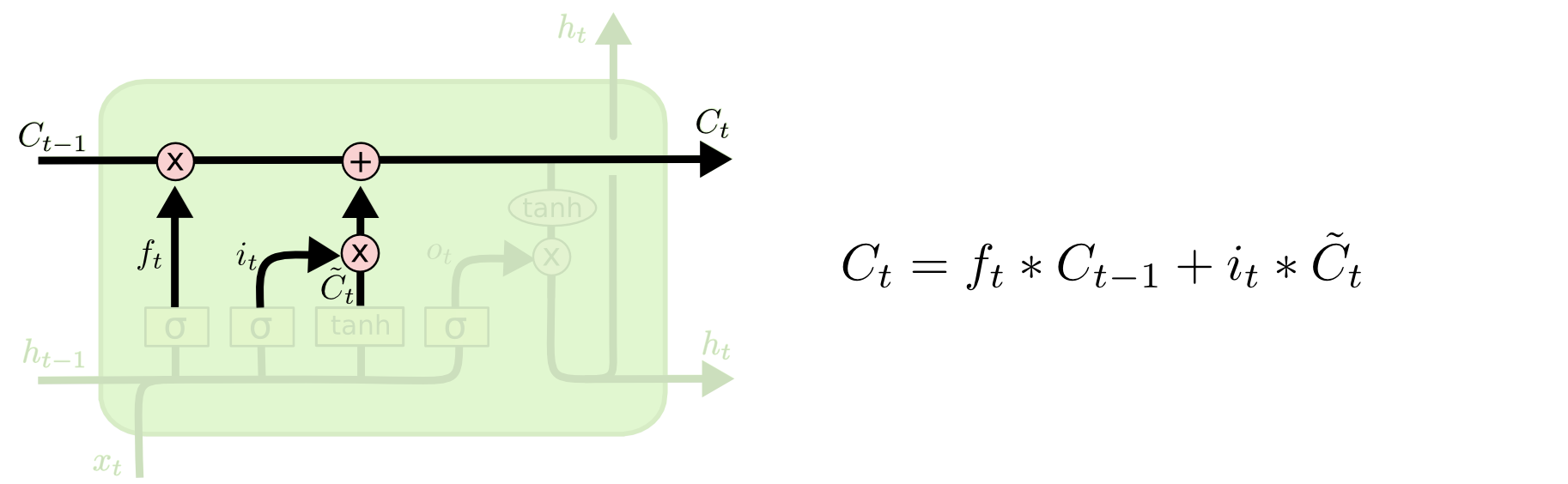
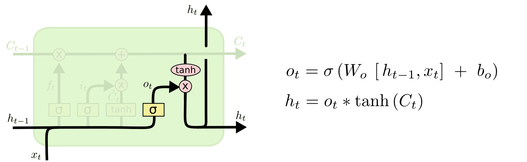
6.2 LSTM
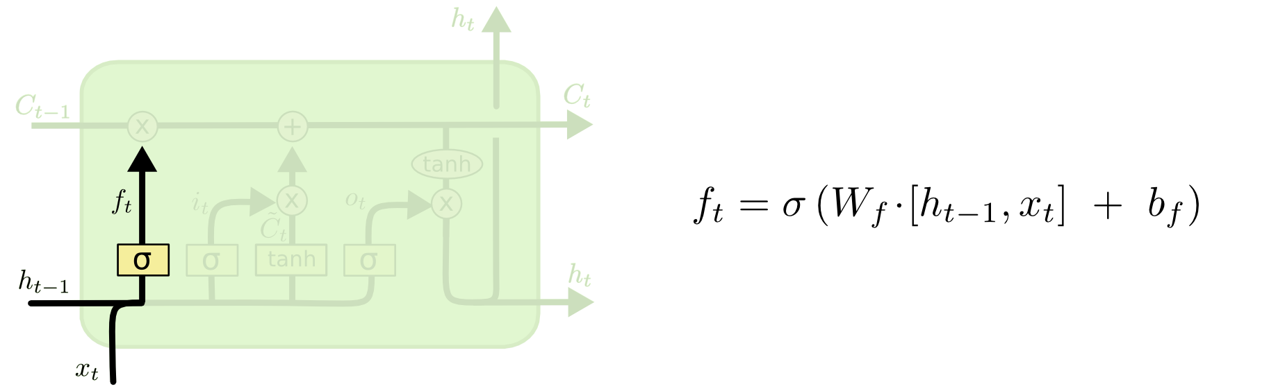
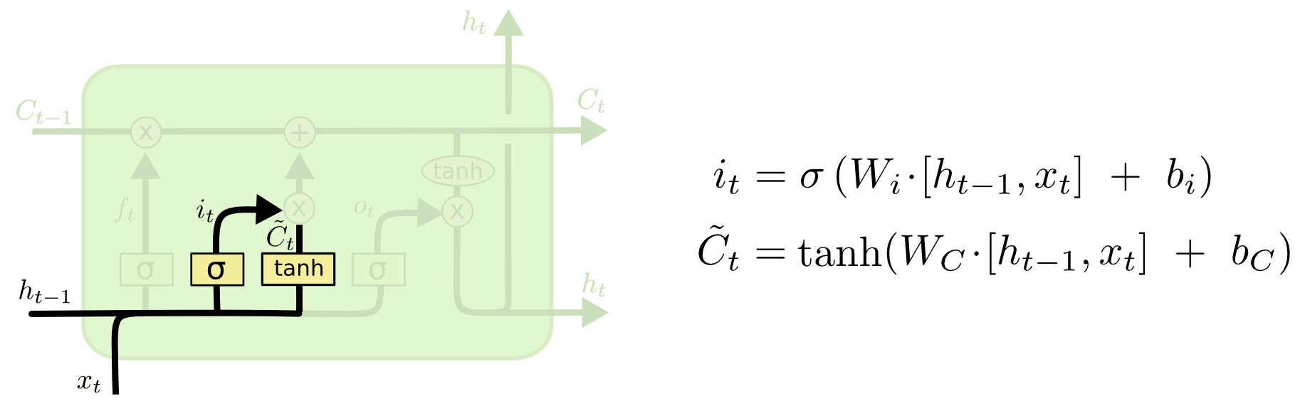
 The above figure shows the repeating module in an LSTM.
Then, in LSTM, each component at step $t$ can be calculated as follows:
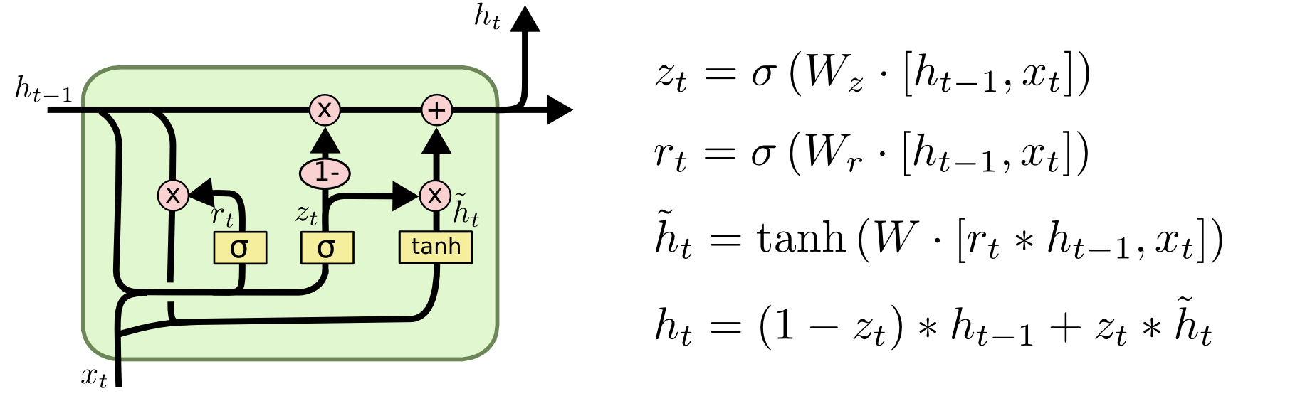
6.3 GRU
GRU combines the forget and input gates into a single “update gate.” It also merges the cell state and hidden state, and makes some other changes. The resulting model is simpler(has less parameters) than standard LSTM models, and has been growing increasingly popular.
6.4 Experiments on IMDB dataset
Referrences:
# import lib
import tensorflow as tf
from tensorflow import keras

import numpy as np

# print(tf.__version__)
# download and explore imdb dataset
imdb = keras.datasets.imdb
# here we use keras api to simplify the downloading and preprocessing process
(train_data, train_labels), (test_data, test_labels) = imdb.load_data(num_words=10000)
# show data num
print("Training entries: {}, labels: {}".format(len(train_data), len(train_labels)))
# show review example, word index
print(train_data[0])
# show different review length
len(train_data[0]), len(train_data[1])
# Convert the integers back to words
# A dictionary mapping words to an integer index
word_index = imdb.get_word_index()

# The first indices are reserved
word_index = {k:(v+3) for k,v in word_index.items()}
word_index["<PAD>"] = 0
word_index["<START>"] = 1
word_index["<UNK>"] = 2  # unknown
word_index["<UNUSED>"] = 3

reverse_word_index = dict([(value, key) for (key, value) in word_index.items()])

def decode_review(text):
    return ' '.join([reverse_word_index.get(i, '?') for i in text])
# show true review example
decode_review(train_data[0])
# prepare the raw data to keras api input format
train_data = keras.preprocessing.sequence.pad_sequences(train_data,
                                                        value=word_index["<PAD>"],
                                                        padding='post',
                                                        maxlen=256)

test_data = keras.preprocessing.sequence.pad_sequences(test_data,
                                                       value=word_index["<PAD>"],
                                                       padding='post',
                                                       maxlen=256)
# show length of of preprared diffrent reviews
len(train_data[0]), len(train_data[1])
# show padded (with zero) review example
print(train_data[0])
decode_review(train_data[0])
# build the model.
def build_model(rnn):
    # input shape is the vocabulary count used for the movie reviews (10,000 words)
    vocab_size = 10000

    model = keras.Sequential()
    model.add(keras.layers.Embedding(vocab_size, 50, input_length=256))
    model.add(keras.layers.Dropout(0.2)) # dropout
    # here we just use the output of the final layer to do the classification work
    model.add(rnn)
    # or if running on a GPU:
    #model.add(keras.layers.CuDNNLSTM(lstm_units))

    # To stack multiple RNN layers, all RNN layers except the last one need
    # to have "return_sequences=True".  An example of using two RNN layers:
    #model.add(keras.layers.LSTM(lstm_units, return_sequences=True))
    #model.add(keras.layers.LSTM(lstm_units))

    model.add(keras.layers.Dense(1, activation='sigmoid'))

    # try using different optimizers and different optimizer configs
    model.compile(loss='binary_crossentropy',
                  optimizer='rmsprop',
                  metrics=['accuracy'])
    print(model.summary())
    return model
print('build LSTM..')
lstm = build_model(keras.layers.LSTM(32))
print('build GRU..')
gru = build_model(keras.layers.GRU(32))
# so short when using keras api!!!
%%time
epochs = 5
validation_split = 0.2

lstm_history = lstm.fit(train_data, train_labels, batch_size=128,
          epochs=epochs,
          validation_split=validation_split)
%%time
gru_history = gru.fit(train_data, train_labels, batch_size=128,
          epochs=epochs,
          validation_split=validation_split)
We can see that GRU is faster than LSTM, then we will compare the accuracy on test set.
# evaluate the model
lstm_scores = lstm.evaluate(test_data, test_labels)
gru_scores = gru.evaluate(test_data, test_labels)
print('lstm accuracy: {}\n gru accuracy: {}'.format(lstm_scores[1], gru_scores[1]))
# see https://github.com/tensorflow/docs/blob/master/site/en/tutorials/keras/basic_text_classification.ipynb,
# the accuracy of naive mlp as follows is 0.87, I have tried a few times but failed to design a good LSTM or GRU
# model = keras.Sequential()
# model.add(keras.layers.Embedding(vocab_size, 16))
# model.add(keras.layers.GlobalAveragePooling1D())
# model.add(keras.layers.Dense(16, activation=tf.nn.relu))
# model.add(keras.layers.Dense(1, activation=tf.nn.sigmoid))
%matplotlib inline
def plot_train_process(history):

    import matplotlib.pyplot as plt

    acc = history.history['acc']
    val_acc = history.history['val_acc']
    loss = history.history['loss']
    val_loss = history.history['val_loss']

    epochs = range(1, len(acc) + 1)

    # "bo" is for "blue dot"
    plt.plot(epochs, loss, 'bo', label='Training loss')
    # b is for "solid blue line"
    plt.plot(epochs, val_loss, 'b', label='Validation loss')
    plt.title('Training and validation loss')
    plt.xlabel('Epochs')
    plt.ylabel('Loss')
    plt.legend()

    plt.show()

    plt.figure()   # new figure

    history_dict = history.history
    acc_values = history_dict['acc']
    val_acc_values = history_dict['val_acc']

    plt.plot(epochs, acc, 'bo', label='Training acc')
    plt.plot(epochs, val_acc, 'b', label='Validation acc')
    plt.title('Training and validation accuracy')
    plt.xlabel('Epochs')
    plt.ylabel('Accuracy')
    plt.legend()

    plt.show()
print('lstm training process: \n')
plot_train_process(lstm_history)
print('gru training process: \n')
plot_train_process(gru_history)


